Figure Candidate Atlas
This atlas makes the visual side of the archive explicit. It separates original scan-derived crops from OCR/PDF-text figure references, then routes each candidate back to the source text and chapter workbench for verification.
Diagram research layer
Original Crops, Candidate Figures, And Verification Routes
Use this page to see what is already visually promoted, what still needs cropping, and where each candidate figure reference appears in the processed corpus.
promoted scan crops
with manifests and checksumsfigure references
OCR/PDF-text candidates needing reviewsources represented
book and report-level visual routingsection-linked candidates
direct text/workbench routesReader Routes
Section titled “Reader Routes”Promoted Original Scan Crops
Section titled “Promoted Original Scan Crops”These are not interpretive redraws. They are documentary scan crops with source-location and checksum records, still awaiting second-pass review before final canonical status.
Radiation, Light and Illumination
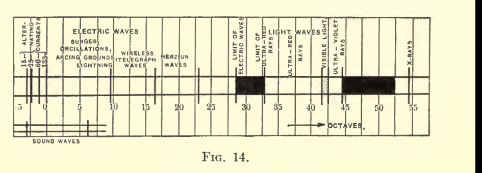
Radiation, Light and Illumination, printed page 18, Fig. 14
Radiation, Light and Illumination
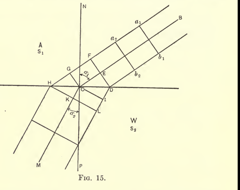
Radiation, Light and Illumination, printed page 22, PDF page 42; Fig. 15
Radiation, Light and Illumination
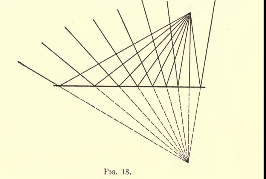
Radiation, Light and Illumination, printed page 28, PDF page 48; Fig. 18
Radiation, Light and Illumination
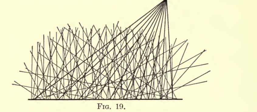
Radiation, Light and Illumination, printed page 29, PDF page 49; Fig. 19
Radiation, Light and Illumination
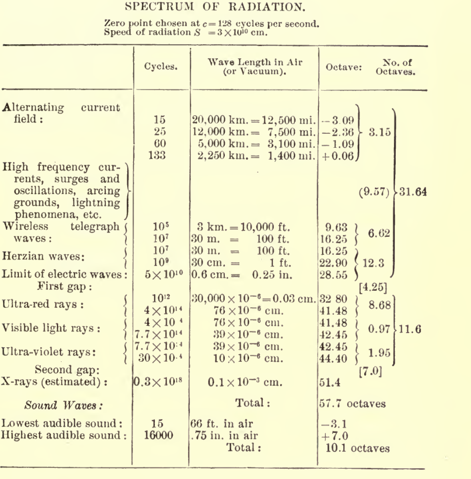
Radiation, Light and Illumination, printed page 17, PDF page 37; Spectrum of Radiation table preceding Fig. 14
Theory and Calculation of Alternating Current Phenomena
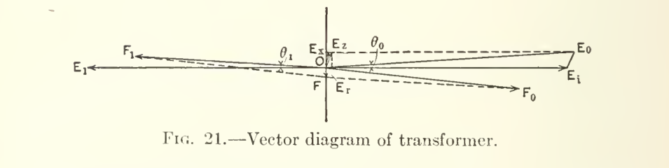
Theory and Calculation of Alternating Current Phenomena, Chapter V, printed page 30, PDF page 58; Fig. 21
Theory and Calculation of Alternating Current Phenomena
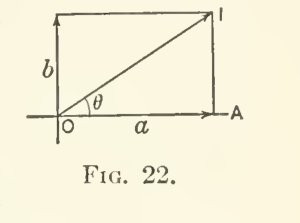
Theory and Calculation of Alternating Current Phenomena, Chapter V, printed page 31, PDF page 59; Fig. 22
Theory and Calculation of Alternating Current Phenomena
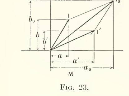
Theory and Calculation of Alternating Current Phenomena, Chapter V, printed page 32, PDF page 60; Fig. 23
Theory and Calculation of Alternating Current Phenomena
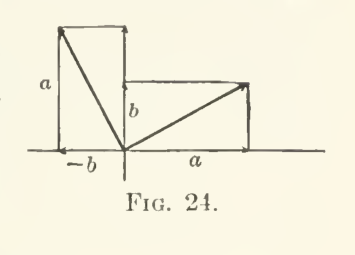
Theory and Calculation of Alternating Current Phenomena, Chapter V, printed page 33, PDF page 61; Fig. 24
Theory and Calculation of Transient Electric Phenomena and Oscillations
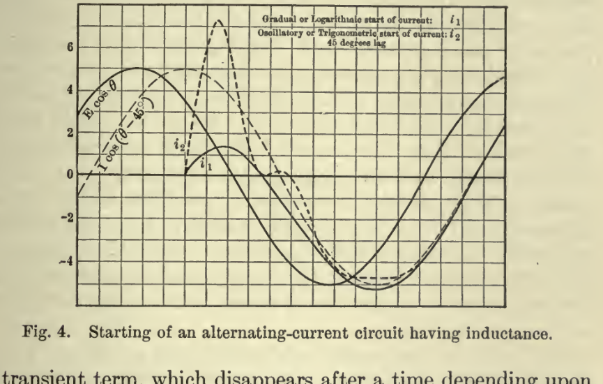
Theory and Calculation of Transient Electric Phenomena and Oscillations, Introduction, printed page 21, PDF page 53; Fig. 4
Theory and Calculation of Transient Electric Phenomena and Oscillations
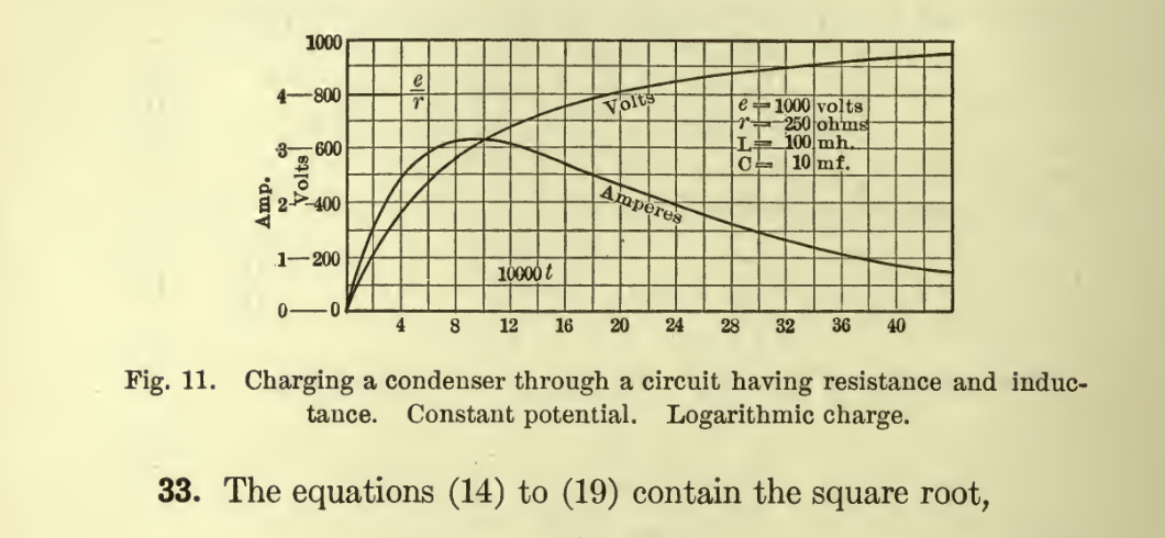
Theory and Calculation of Transient Electric Phenomena and Oscillations, Condenser Charge and Discharge, printed page 52, PDF page 84; Fig. 11
Theory and Calculation of Transient Electric Phenomena and Oscillations
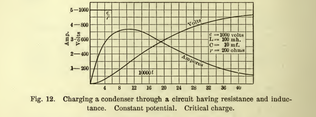
Theory and Calculation of Transient Electric Phenomena and Oscillations, Condenser Charge and Discharge, printed page 58, PDF page 90; Fig. 12
Theory and Calculation of Transient Electric Phenomena and Oscillations
Theory and Calculation of Transient Electric Phenomena and Oscillations, Condenser Charge and Discharge, printed page 61, PDF page 93; Fig. 13
Theory and Calculation of Transient Electric Phenomena and Oscillations
Theory and Calculation of Transient Electric Phenomena and Oscillations, Condenser Charge and Discharge, printed page 62, PDF page 94; Fig. 14
Theory and Calculation of Transient Electric Phenomena and Oscillations
Theory and Calculation of Transient Electric Phenomena and Oscillations, Condenser Charge and Discharge, printed page 65, PDF page 97; Fig. 15
Source-Level Figure Coverage
Section titled “Source-Level Figure Coverage”Candidate Figure References By Source
Section titled “Candidate Figure References By Source”The rows below are OCR/PDF-text candidates. Captions may include nearby text, line breaks, OCR mistakes, or partial figure labels. Treat them as a locator for scan review, not a final caption.
Theory and Calculation of Alternating Current Phenomena 145 candidate figure references - 4 promoted crops
| Figure | OCR/PDF-Text Caption Candidate | Location | Section | Open | Status |
|---|---|---|---|---|---|
| Fig. 6 | maximum variation of the sine is equal to the variation of the Fig. 6. Fig. 7. | line 1864 | Chapter 2: Instantaneous Values And Integral Values | text - workbench | needs-verification |
| Fig. 7 | Fig. 6. Fig. 7. corresponding arc, and consequently the maximum variation of | line 1867 | Chapter 2: Instantaneous Values And Integral Values | text - workbench | needs-verification |
| Fig. 10 | 21 Fig. 10. phase angle — /3’ = — (a’ — ??]) = 10 A, and the equations of | line 2262 | Chapter 4: Vector Representation | text - workbench | needs-verification |
| Fig. 16 | ^E, Fig. 16. Fig. 17. | line 2534 | Chapter 4: Vector Representation | text - workbench | needs-verification |
| Fig. 17 | Fig. 16. Fig. 17. the current by the angle, Q. The voltage consumed by the resist- | line 2537 | Chapter 4: Vector Representation | text - workbench | needs-verification |
| Fig. 19 | Ei-< «; Fig. 19. The primary impressed e.m.f., Ep, must thus consist of the three components OEi, OEr, and OE^, and is, therefore, their | line 2704 | Chapter 4: Vector Representation | text - workbench | needs-verification |
| Fig. 24 | 33 Fig. 24. polar coordinates by a vector of opposite direction, and denoted | line 2937 | Chapter 5: Symbolic Method | text - workbench | needs-verification |
| Fig. 25 | ,,U— — L Fig. 25. Fig. 26. | line 3289 | Chapter 6: Topographic Method | text - workbench | needs-verification |
| Fig. 26 | Fig. 25. Fig. 26. in the opposite direction, from terminal B to terminal A in op- | line 3292 | Chapter 6: Topographic Method | text - workbench | needs-verification |
| Fig. 29 | NON-INDUCTIVE LOAD Fig. 29. Fig. 30. | line 3392 | Chapter 6: Topographic Method | text - workbench | needs-verification |
| Fig. 30 | Fig. 29. Fig. 30. these currents are represented in Fig. 29 by the vectors 01 1 = | line 3395 | Chapter 6: Topographic Method | text - workbench | needs-verification |
| Fig. 31 | CAPACIir AND RESISTANCE Fig. 31. Fig. 32. | line 3446 | Chapter 6: Topographic Method | text - workbench | needs-verification |
| Fig. 32 | Fig. 31. Fig. 32. triangle, Ei^E^^Ez^, the voltages at the receiver’s circuit, Ei, E2, | line 3449 | Chapter 6: Topographic Method | text - workbench | needs-verification |
| Fig. 33 | RESISTANCE AND LEAKAGE Fig. 33. 16 I TRANSMISSION | line 3554 | Chapter 6: Topographic Method | text - workbench | needs-verification |
| Fig. 34 | 90” LAG Fig. 34. and generator currents, /i”, 72°, I^, over the topographical char- | line 3566 | Chapter 6: Topographic Method | text - workbench | needs-verification |
| Fig. 35 | RESISTANCE AND LEAKAGE Fig. 35. their difference of phase are plotted in Fig. 35 in rectangular | line 3605 | Chapter 6: Topographic Method | text - workbench | needs-verification |
| Fig. 37 | represented by an increase of angle B in counter-clockwise rota- FiG. 37 tion. That is, the positive direction, or increase of time, is | line 3691 | Chapter 7: Polar Coordinates And Polar Diagrams | text - workbench | needs-verification |
| Fig. 41 | ^i Fig. 41. Fig. 42. | line 3828 | Chapter 7: Polar Coordinates And Polar Diagrams | text - workbench | needs-verification |
| Fig. 42 | Fig. 41. Fig. 42. then appear in the vector representation of the time diagram or | line 3831 | Chapter 7: Polar Coordinates And Polar Diagrams | text - workbench | needs-verification |
| Fig. 43 | E^-^ Fig. 43. Fig. 45. | line 3856 | Chapter 7: Polar Coordinates And Polar Diagrams | text - workbench | needs-verification |
| Fig. 45 | Fig. 43. Fig. 45. lagging behind the voltage: | line 3859 | Chapter 7: Polar Coordinates And Polar Diagrams | text - workbench | needs-verification |
| Fig. 46 | then means: Fig. 46. POLAR COORDINATES AND POLAR DIAGRAMS 51 | line 3872 | Chapter 7: Polar Coordinates And Polar Diagrams | text - workbench | needs-verification |
| Fig. 48 | ^ Fig. 48. R’ | line 4049 | Chapter 7: Polar Coordinates And Polar Diagrams | text - workbench | needs-verification |
| Fig. 49 | 7 1.8 Fig. 49. The sign in the complex expression of admittance is always opposite to that of impedance; this is obvious, since if the cur- | line 4618 | Chapter 8: Admittance, Conductance, Susceptance | text - workbench | needs-verification |
| Fig. 51 | Eo E Fig. 51. M | line 5008 | Chapter 9: Circuits Containing Resistance, Inductive Reactance, And Condensive Reactance | text - workbench | needs-verification |
| Fig. 52 | Eo Fig. 52. Fig. 53. | line 5025 | Chapter 9: Circuits Containing Resistance, Inductive Reactance, And Condensive Reactance | text - workbench | needs-verification |
| Fig. 53 | Fig. 52. Fig. 53. 2. Reactance in Series with a Circuit | line 5028 | Chapter 9: Circuits Containing Resistance, Inductive Reactance, And Condensive Reactance | text - workbench | needs-verification |
| Fig. 54 | ohms inductance-’— reactance-^condensance Fig. 54. E^, are shown for various conditions of a receiver circuit and | line 5409 | Chapter 9: Circuits Containing Resistance, Inductive Reactance, And Condensive Reactance | text - workbench | needs-verification |
| Fig. 55 | 0 Fig. 55. Fig. 56. | line 5474 | Chapter 9: Circuits Containing Resistance, Inductive Reactance, And Condensive Reactance | text - workbench | needs-verification |
| Fig. 56 | Fig. 55. Fig. 56. Fig. 57. | line 5477 | Chapter 9: Circuits Containing Resistance, Inductive Reactance, And Condensive Reactance | text - workbench | needs-verification |
| Fig. 57 | Fig. 56. Fig. 57. is, the current and e.m.f. in the supply circuit are in phase with | line 5480 | Chapter 9: Circuits Containing Resistance, Inductive Reactance, And Condensive Reactance | text - workbench | needs-verification |
| Fig. 58 | ^w=+90 80 70 60 50 40 30 20 10 0 10 20 30 40 50 60 70 80 90 degrees lag-«- phase difference in consumer circuit-*- lead Fig. 58. In Figs. 59 and 60, the same curves are plotted as in Fig. 58, but in Fig. 59 with the reactance, x, of the receiver circuit as | line 5572 | Chapter 9: Circuits Containing Resistance, Inductive Reactance, And Condensive Reactance | text - workbench | needs-verification |
| Fig. 59 | +1 +.9 +.8 +.7 +.6 +.5 +.4 +.3 +.2 +.1 0 -.1 -.2 -.3 -.4 -.5 -.6 reactance of consumer circuit Fig. 59. -.7 -.8 -.9-10 | line 5894 | Chapter 9: Circuits Containing Resistance, Inductive Reactance, And Condensive Reactance | text - workbench | needs-verification |
| Fig. 60 | _ resistance of . consumer circuit Fig. 60. ,7 .6 .5 .4 .3 .2 .1 .0 | line 6052 | Chapter 9: Circuits Containing Resistance, Inductive Reactance, And Condensive Reactance | text - workbench | needs-verification |
| Fig. 61 | 1. .9 .8 .7 .6 .5 ,4 .3 .2 .1 0 -.1 -.2 -.3 -.1 -.5 -.6 -.7 -.8 -.9-L X — ^ Fig. 61. E | line 6302 | Chapter 9: Circuits Containing Resistance, Inductive Reactance, And Condensive Reactance | text - workbench | needs-verification |
| Fig. 62 | tro Fig. 62. Fig. 63. | line 6333 | Chapter 9: Circuits Containing Resistance, Inductive Reactance, And Condensive Reactance | text - workbench | needs-verification |
| Fig. 63 | Fig. 62. Fig. 63. 72 | line 6336 | Chapter 9: Circuits Containing Resistance, Inductive Reactance, And Condensive Reactance | text - workbench | needs-verification |
| Fig. 65 | loss of power. Fig. 65. Then, if Eo = impressed e.m.f., the current in receiver circuit is | line 6409 | Chapter 9: Circuits Containing Resistance, Inductive Reactance, And Condensive Reactance | text - workbench | needs-verification |
| Fig. 67 | 1 Fig. 67. 5. Constant Potential — Constant-current Transformation | line 6939 | Chapter 9: Circuits Containing Resistance, Inductive Reactance, And Condensive Reactance | text - workbench | needs-verification |
| Fig. 68 | supply, and inversely. Fig. 68 The generation of alternating-current electric power almost always takes place at constant potential. For some purposes, | line 6973 | Chapter 9: Circuits Containing Resistance, Inductive Reactance, And Condensive Reactance | text - workbench | needs-verification |
| Fig. 72 | 0 Fig. 72. .03 ,03 M. .05 .00 .07 .OS | line 8597 | Chapter 10: Resistance And Reactance Of Transmission | text - workbench | needs-verification |
| Fig. 76 | » Fig. 76. 10 20 30 10 50 60 7.0 .80 90 100 | line 9705 | Chapter 10: Resistance And Reactance Of Transmission | text - workbench | needs-verification |
| Fig. 77 | AMPERES LOAD « l Fig. 77. and the leading quadrature component of current required to compensate for the line reactance x at maximum current, im, is | line 10085 | Chapter 11: Phase Control | text - workbench | needs-verification |
| Fig. 78 | ::} Fig. 78. 87. Equation (28) shows that there are two values of x: Xi and X2; and corresponding thereto two values of 60:^01 and 602, | line 10552 | Chapter 11: Phase Control | text - workbench | needs-verification |
| Fig. 81 | ^ Fig. 81. The general character of these current waves is, that the maxi- | line 11510 | Chapter 12: Effective Resistance And Reactance | text - workbench | needs-verification |
| Fig. 82 | then Fig. 82. — X^ | line 12025 | Chapter 12: Effective Resistance And Reactance | text - workbench | needs-verification |
| Fig. 86 | n = NUMBER OF TURNS Fig. 86. 350 | line 12600 | Chapter 12: Effective Resistance And Reactance | text - workbench | needs-verification |
| Fig. 87 | / = FREQUENCY Fig. 87. 400 | line 12686 | Chapter 12: Effective Resistance And Reactance | text - workbench | needs-verification |
| Fig. 88 | 200 250 Fig. 88. 300 | line 12813 | Chapter 12: Effective Resistance And Reactance | text - workbench | needs-verification |
| Fig. 89 | /=CYCLES Fig. 89. 300 | line 12940 | Chapter 12: Effective Resistance And Reactance | text - workbench | needs-verification |
| Fig. 90 | n=NUMBER OF TURNS Fig. 90. 350 | line 13034 | Chapter 12: Effective Resistance And Reactance | text - workbench | needs-verification |
| Fig. 92 | magnetic flux inclosed by the zone is SuV. Fig. 92. Hence, the e.m.f. generated in this zone is | line 13742 | Chapter 13: Foucault Or Eddy Currents | text - workbench | needs-verification |
| Fig. 93 | 93. Fig. 93. 110. Demagnetizing, or screening effect of eddy currents. | line 13860 | Chapter 13: Foucault Or Eddy Currents | text - workbench | needs-verification |
| Fig. 94 | du Fig. 94. The current inclosed by this zone is /„ | line 14074 | Chapter 13: Foucault Or Eddy Currents | text - workbench | needs-verification |
| Fig. 96 | ^ m Fig. 96. )J | line 15113 | Chapter 14: Dielectric Losses | text - workbench | needs-verification |
| Fig. 97 | ’ m Fig. 97. throughout the field section, but the voltage gradient in the | line 15131 | Chapter 14: Dielectric Losses | text - workbench | needs-verification |
| Fig. 98 | do so. Fig. 98. Fig. 99. | line 15252 | Chapter 14: Dielectric Losses | text - workbench | needs-verification |
| Fig. 99 | Fig. 98. Fig. 99. h’5 | line 15255 | Chapter 14: Dielectric Losses | text - workbench | needs-verification |
| Fig. 100 | JTTTTTTTTTTTTTTTTTTTTTTT- Fig. 100. In this case the intensity as well as phase of the current, and consequently of the counter e.m.f. of inductive reactance and | line 15474 | Chapter 15: Distributed Capacity, Inductance, Resistance, And Leakage | text - workbench | needs-verification |
| Fig. 101 | iEo Fig. 101. Denoting in Fig. 101. | line 15606 | Chapter 15: Distributed Capacity, Inductance, Resistance, And Leakage | text - workbench | needs-verification |
| Fig. 102 | phase (for convenience, as intensities, the effective values are Fig. 102. used throughout), assuming its phase as the downwards vertical; that is, counting the time from the moment where the rising | line 16703 | Chapter 17: The Alternating-Current Transformer | text - workbench | needs-verification |
| Fig. 103 | Eo Fig. 103. Figs. 103 to 109 give the polar diagram of a transformer having | line 16830 | Chapter 17: The Alternating-Current Transformer | text - workbench | needs-verification |
| Fig. 104 | ALTERNATING-CURRENT TRANSFORMER 193 Fig. 104. ./ ^^0 | line 16861 | Chapter 17: The Alternating-Current Transformer | text - workbench | needs-verification |
| Fig. 105 | ./ ^^0 Fig. 105. 13 | line 16867 | Chapter 17: The Alternating-Current Transformer | text - workbench | needs-verification |
| Fig. 106 | 13 Fig. 106. 194 ALTERNATING-CURRENT PHENOMENA | line 16873 | Chapter 17: The Alternating-Current Transformer | text - workbench | needs-verification |
| Fig. 107 | 194 ALTERNATING-CURRENT PHENOMENA Fig. 107. Fia. 108. | line 16879 | Chapter 17: The Alternating-Current Transformer | text - workbench | needs-verification |
| Fig. 113 | gram of Fig. 110, the diagrams for the constant primary im- FiG. 113. pressed e.m.f. (Fig. Ill), and for constant secondary terminal | line 16908 | Chapter 17: The Alternating-Current Transformer | text - workbench | needs-verification |
| Fig. 114 | Circuit Fig. 114. 152. Separating now the internal secondary impedance from the external secondary impedance, or the impedance of the | line 17408 | Chapter 17: The Alternating-Current Transformer | text - workbench | needs-verification |
| Fig. 116 | ”El Fig. 116. It is obvious, therefore, that if the transformer contains sev- | line 17474 | Chapter 17: The Alternating-Current Transformer | text - workbench | needs-verification |
| Fig. 117 | of admittance Yq. Thus, double transformation will be represented by diagram. Fig. 117. With this the discussion of the alternate-current transformer ends, by becoming identical with that of a divided circuit con- | line 17508 | Chapter 17: The Alternating-Current Transformer | text - workbench | needs-verification |
| Fig. 118 | is the angle of secondary lag. Fig. 118. The secondary m.m.f., OGi, is in the direction of the vector, | line 18102 | Chapter 18: Polyphase Induction Motors | text - workbench | needs-verification |
| Fig. 119 | determined thus, Fig. 119. Let | line 18133 | Chapter 18: Polyphase Induction Motors | text - workbench | needs-verification |
| Fig. 120 | AMPERES Fig. 120. 90 | line 19057 | Chapter 18: Polyphase Induction Motors | text - workbench | needs-verification |
| Fig. 121 | AMPERES Fig. 121. 250 | line 19500 | Chapter 18: Polyphase Induction Motors | text - workbench | needs-verification |
| Fig. 122 | . Fig. 122. On the same figure is shown the current per line, in dotted lines, with the verticals or torque as abscissas, and the hori- | line 19753 | Chapter 18: Polyphase Induction Motors | text - workbench | needs-verification |
| Fig. 123 | DO Fig. 123. hence, the efficiency is, Pi_ ^ ai (1 - s) | line 20132 | Chapter 18: Polyphase Induction Motors | text - workbench | needs-verification |
| Fig. 124 | 0 Fig. 124. and the apparent torque efficiency,^ | line 20407 | Chapter 18: Polyphase Induction Motors | text - workbench | needs-verification |
| Fig. 125 | KX) Fig. 125. voltage will rise until by magnetic saturation in the induction generator its power-factor has fallen to equality with that of | line 20763 | Chapter 19: Induction Generators | text - workbench | needs-verification |
| Fig. 126 | )00 Fig. 126. the efficiency. | line 21111 | Chapter 19: Induction Generators | text - workbench | needs-verification |
| Fig. 127 | 0 Fig. 127. and the terminal voltage at the synchronous motor, | line 21509 | Chapter 19: Induction Generators | text - workbench | needs-verification |
| Fig. 128 | Eo.U.Yj Fig. 128. shading coil is commonly used) is the monocyclic starting device. It consists in producing externally to the motor a system of | line 22028 | Chapter 20: Single-Phase Induction Motors | text - workbench | needs-verification |
| Fig. 129 | former; hence fixed in space relative to the field m.m.f., or uni- FiG. 129. directional; but pulsating in a single-phase alternator. In the polyphase alternator, when evenly loaded or balanced, the result- | line 22319 | Chapter 21: Alternating-Current Generator | text - workbench | needs-verification |
| Fig. 130 | be assumed as constant. Fig. 130. The relative position of the armature m.m.f. with respect to | line 22363 | Chapter 21: Alternating-Current Generator | text - workbench | needs-verification |
| Fig. 131 | excitation, increases the voltage; with lagging current it weakens Fig. 131. the field, and thereby decreases the voltage in a generator. Ob- viously, the opposite holds for a synchronous motor, in which the | line 22406 | Chapter 21: Alternating-Current Generator | text - workbench | needs-verification |
| Fig. 139 | phase, the virtual generated e.m.f. Fig. 139. The armature self-induction consumes an e.m.f., OE3, 90° | line 24075 | Chapter 22: Armature Reactions Of Alternators | text - workbench | needs-verification |
| Fig. 140 | OFi’, and OF” = OFi”. Fig. 140. Let now (P’ = permeance of the field magnetic circuit; | line 24385 | Chapter 22: Armature Reactions Of Alternators | text - workbench | needs-verification |
| Fig. 141 | actual value of the field onward Fig. 141. -as shown by Fig, 141. | line 24490 | Chapter 22: Armature Reactions Of Alternators | text - workbench | needs-verification |
| Fig. 142 | AMPERES Fig. 142. an alternator of pulsating synchronous reactance, the wave-shape of the machine changes more or less with the load and the char- | line 25128 | Chapter 22: Armature Reactions Of Alternators | text - workbench | needs-verification |
| Fig. 143 | mnrmnmnwv Fig. 143. allel; as, for instance, by the arrangement shown in Fig. 143, | line 25260 | Chapter 23: Synchronizing Alternators | text - workbench | needs-verification |
| Fig. 144 | nal admittance of the second machine. Fig. 144. Then, er + e’r = al^• | line 25324 | Chapter 23: Synchronizing Alternators | text - workbench | needs-verification |
| Fig. 145 | impedance of the line, and the e.m.f., Es^E = E4, consumed by Fig. 145. the impedance of the generator. Hence, dividing the opposite | line 25805 | Chapter 24: Synchronous Motor | text - workbench | needs-verification |
| Fig. 146 | 304 ALTERNATING-CURRENT PHENOMENA Fig. 146. Fig. 147. | line 25830 | Chapter 24: Synchronous Motor | text - workbench | needs-verification |
| Fig. 147 | Fig. 146. Fig. 147. SYNCHRONOUS MOTOR | line 25833 | Chapter 24: Synchronous Motor | text - workbench | needs-verification |
| Fig. 148 | 305 Fig. 148. Fig. 149. | line 25842 | Chapter 24: Synchronous Motor | text - workbench | needs-verification |
| Fig. 149 | Fig. 148. Fig. 149. 20 | line 25845 | Chapter 24: Synchronous Motor | text - workbench | needs-verification |
| Fig. 150 | have < EiOE = 90°, Ei = Eo, thus: OEi = EEo = OEo = E^r, Fig. 150. Fig. 151. | line 25963 | Chapter 24: Synchronous Motor | text - workbench | needs-verification |
| Fig. 151 | Fig. 150. Fig. 151. that is, EEi = 2 £“0. That means the characteristic curve, Ci, is | line 25966 | Chapter 24: Synchronous Motor | text - workbench | needs-verification |
| Fig. 152 | shown in Fig. 151. Fig. 152. If El < Eo, at small Eo — Ei, H can be below the zero line, | line 25997 | Chapter 24: Synchronous Motor | text - workbench | needs-verification |
| Fig. 154 | of the cases the current is leading, in the other lagging. Fig. 154. In Figs. 155 to 158 are shown diagrams, giving the points | line 26150 | Chapter 24: Synchronous Motor | text - workbench | needs-verification |
| Fig. 155 | 20 < / < 30 Fig. 155. Fig. 156. | line 26186 | Chapter 24: Synchronous Motor | text - workbench | needs-verification |
| Fig. 156 | Fig. 155. Fig. 156. Fig. 157. | line 26188 | Chapter 24: Synchronous Motor | text - workbench | needs-verification |
| Fig. 157 | Fig. 156. Fig. 157. Fig. 158. | line 26190 | Chapter 24: Synchronous Motor | text - workbench | needs-verification |
| Fig. 158 | Fig. 157. Fig. 158. As seen, the permissible value of counter e.m.f., Ei, and of | line 26192 | Chapter 24: Synchronous Motor | text - workbench | needs-verification |
| Fig. 159 | e=*iie— -i Fig. 159. Fig. 160. | line 26540 | Chapter 24: Synchronous Motor | text - workbench | needs-verification |
| Fig. 160 | Fig. 159. Fig. 160. This equation shows that, at given impressed e.m.f., eo, and | line 26543 | Chapter 24: Synchronous Motor | text - workbench | needs-verification |
| Fig. 161 | / = er + zH- — co^ ± 2 xie^ = 0; Fig. 161. by the condition, | line 26833 | Chapter 24: Synchronous Motor | text - workbench | needs-verification |
| Fig. 162 | MO ma ‘i&bo ~ 2000 2500 -^000 saoo iooo taoo eooo ewo Fig. 162. Minimum counter e.m.f. point of this curve, | line 27147 | Chapter 24: Synchronous Motor | text - workbench | needs-verification |
| Fig. 163 | 2500 Volts Fig. 163. 3000 | line 27254 | Chapter 24: Synchronous Motor | text - workbench | needs-verification |
| Fig. 164 | X = reactance of the circuit between counter e.m.f., e, and im- FiG. 164. pressed e.m.f., eo, OEr = iiv = e.m.f. consumed by resistance, OEj: = iix = e.m.f. consumed by reactance of the power com- | line 27404 | Chapter 24: Synchronous Motor | text - workbench | needs-verification |
| Fig. 165 | 200 400 COO SOO 1000 1200 1100 1600 1800 2000 2200 2400 2000^2800 8000 3200 S400 3CO0 SSOO 4000 4200 VOLTS = e Fig. 165. 248. As illustrations are plotted, in Fig. 165, curves giving the current, i, as function of the counter or nominal generated e.m.f., | line 27859 | Chapter 24: Synchronous Motor | text - workbench | needs-verification |
| Fig. 166 | KILOWATTS Fig. 166. 1 1 | line 28114 | Chapter 24: Synchronous Motor | text - workbench | needs-verification |
| Fig. 168 | KILOWATTS Fig. 168. 229. I. hoad Curves of Synchronous Motor. | line 28468 | Chapter 24: Synchronous Motor | text - workbench | needs-verification |
| Fig. 169 | KILOWATTS Fig. 169. For low values of e (e = 1600, under excitation, Fig. 166), | line 28681 | Chapter 24: Synchronous Motor | text - workbench | needs-verification |
| Fig. 170 | 600 600 KILOWATTS Fig. 170. It is interesting that at e = 2180, the power-factor is practi- | line 28903 | Chapter 24: Synchronous Motor | text - workbench | needs-verification |
| Fig. 171 | KILOWATTS Fig. 171. that at the same impressed voltage, with the same current input | line 29234 | Chapter 24: Synchronous Motor | text - workbench | needs-verification |
| Fig. 172 | 1 180 Fig. 172. Even with an unsymmetrical distribution of the magnetic flux in the air-gap, the e.m.f. wave generated in a full-pitch | line 29650 | Chapter 25: Distortion Of Wave-Shape And Its Causes | text - workbench | needs-verification |
| Fig. 173 | 180 Fig. 173. magnetic reluctance, or its reciprocal, the magnetic reactance of the circuit. In consequence thereof the magnetism per field- | line 29845 | Chapter 25: Distortion Of Wave-Shape And Its Causes | text - workbench | needs-verification |
| Fig. 178 | ’ Fig. 178. tage drops with the further increase of current, and then rises again with the decreasing current, until at C, the intersection | line 31252 | Chapter 25: Distortion Of Wave-Shape And Its Causes | text - workbench | needs-verification |
| Fig. 179 | 1 Fig. 179. flux and the current, therefore, cannot both be sine waves; if the magnetic flux and therefore the generated e.m.f. are sine waves, | line 31517 | Chapter 25: Distortion Of Wave-Shape And Its Causes | text - workbench | needs-verification |
| Fig. 180 | -B Fig. 180. the e.m.f., e = J? sin </>, and a wattless component, i” , in quadra- | line 31654 | Chapter 25: Distortion Of Wave-Shape And Its Causes | text - workbench | needs-verification |
| Fig. 181 | where Fig. 181. c„ = \/a„2 + 6n^, 6„ | line 31840 | Chapter 25: Distortion Of Wave-Shape And Its Causes | text - workbench | needs-verification |
| Fig. 182 | \v Fig. 182. B. Sine Wave of Current | line 31959 | Chapter 25: Distortion Of Wave-Shape And Its Causes | text - workbench | needs-verification |
| Fig. 183 | y Fig. 183. As seen, with a sine wave of current traversing an iron-clad reactance, the e.m.f. wave is very greatly distorted, and the | line 32214 | Chapter 25: Distortion Of Wave-Shape And Its Causes | text - workbench | needs-verification |
| Fig. 184 | a three-phase system with a sine wave of e.m.f. between the lines, the curves of exciting current, magnetic flux and voltage per transformer, or between lines and neutral, are constructed in Fig. 184. i is the exciting current of the transformer, and contains all the harmonics, except the third and its multiples. It is given | line 32390 | Chapter 25: Distortion Of Wave-Shape And Its Causes | text - workbench | needs-verification |
| Fig. 185 | 4i’ Fig. 185. triple and the quintuple harmonic upon the fundamental sine wave. | line 32554 | Chapter 26: Effects Of Higher Harmonics | text - workbench | needs-verification |
| Fig. 186 | ft Fig. 186. As seen, the effect of the triple harmonic is, in the first figure, to flatten the zero values and point the maximum values of the | line 32594 | Chapter 26: Effects Of Higher Harmonics | text - workbench | needs-verification |
| Fig. 191 | 0 Fig. 191. of the harmonic, and the winding of the motor primary. Thus, | line 34764 | Chapter 27: Symbolic Representation Of General Alternating Waves | text - workbench | needs-verification |
| Fig. 193 | interlinked system. Fig. 193. The four-phase system as derived by connecting four equi- distant points of a continuous-current armature with four | line 34858 | Chapter 28: General Polyphase Systems | text - workbench | needs-verification |
| Fig. 194 | ^<MS^iB>^ 4 Fig. 194. The three-phase system, consisting of three e.m.fs. displaced by one-third of a period, is used exclusively as interlinked system. | line 34897 | Chapter 28: General Polyphase Systems | text - workbench | needs-verification |
| Fig. 195 | —E nmTswusvsvrno- Fig. 195. a three-phase system, in the alternating supply circuit of large synchronous converters. | line 34916 | Chapter 28: General Polyphase Systems | text - workbench | needs-verification |
| Fig. 208 | ^ Fig. 208. 2. The ring connection, represented diagrammatically in Fig. | line 35765 | Chapter 31: Interlinked Polyphase Systems | text - workbench | needs-verification |
| Fig. 209 | 1 Fig. 209. system. In a three-phase system this connection is called the | line 35796 | Chapter 31: Interlinked Polyphase Systems | text - workbench | needs-verification |
| Fig. 210 | nm Fig. 210. The reverse thereof, or the Y-delta connection, is undesirable on unbalanced load, since it gives what has been called a “float- | line 36262 | Chapter 32: Transformation Of Polyphase Systems | text - workbench | needs-verification |
| Fig. 211 | T Fig. 211. and (3) can be operated in parallel with each other, and with the | line 36354 | Chapter 32: Transformation Of Polyphase Systems | text - workbench | needs-verification |
| Fig. 212 | mm) mu Fig. 212. by the internal impedance of the transformers. It is convenient | line 36370 | Chapter 32: Transformation Of Polyphase Systems | text - workbench | needs-verification |
| Fig. 213 | 1 Fig. 213. phase and inverted three-phase or polyphase monocychc, by two transformers, the secondary of one being reversed regarding its | line 36404 | Chapter 32: Transformation Of Polyphase Systems | text - workbench | needs-verification |
| Fig. 214 | CMT\ rWFl Fig. 214. of the transformers contain two equal and independent (or inter- linked) coils, the three-phase sides two coils with the ratio of | line 36420 | Chapter 32: Transformation Of Polyphase Systems | text - workbench | needs-verification |
| Fig. 215 | I 2 Fig. 215. ‘3 ‘2 ‘3 | line 36448 | Chapter 32: Transformation Of Polyphase Systems | text - workbench | needs-verification |
| Fig. 216 | formation from three-phase to six-phase, shown in Fig. 216. It Fig. 216. is analogous to (7), the delta connection merely being replaced | line 36458 | Chapter 32: Transformation Of Polyphase Systems | text - workbench | needs-verification |
| Fig. 217 | I I Fig. 217. The primaries in 9 and 10 may be connected either delta or F, | line 36487 | Chapter 32: Transformation Of Polyphase Systems | text - workbench | needs-verification |
| Fig. 218 | ,^-’-’ ^^ Fig. 218. The voltage between any two terminals e^ and e^ then is: e.7fc = ei — ek ’ (1) | line 37147 | Chapter 34: Metering Of Polyphase Circuit | text - workbench | needs-verification |
| Fig. 219 | -0- FiG. 219. Thus, if Fig. 220 denotes a general three-wire, three-phase sys- tem, with the voltages and currents in the three phases: | line 37331 | Chapter 34: Metering Of Polyphase Circuit | text - workbench | needs-verification |
| Fig. 220 | •3, ‘3 Fig. 220. The voltages may be unequal in sizes and under unequal angles, by a distortion of the three-phase triangle, but it must be: | line 37344 | Chapter 34: Metering Of Polyphase Circuit | text - workbench | needs-verification |
| Fig. 221 | -OD- Fig. 221. system, if the current lags, the two wattmeter coils do not read alike, as the voltmeter coil in the one lags by the angle of lag of | line 37399 | Chapter 34: Metering Of Polyphase Circuit | text - workbench | needs-verification |
| Fig. 222 | -0- FiG. 222. In a four- wire, three-phase system, the connection of the two | line 37441 | Chapter 34: Metering Of Polyphase Circuit | text - workbench | needs-verification |
Radiation, Light and Illumination 98 candidate figure references - 5 promoted crops
| Figure | OCR/PDF-Text Caption Candidate | Location | Section | Open | Status |
|---|---|---|---|---|---|
| Fig. 1 | tion, the time at which the moon M should disappear from sight, FIG. 1. when seen from the earth E, by passing behind Jupiter, 7 (Fig. 1), could be exactly calculated. It was found, however, that some- | line 656 | Lecture 1: Nature And Different Forms Of Radiation | text - workbench | needs-verification |
| Fig. 2 | 5_MOE_S FIG. 2. direction the light reappears. If the disk is slowly revolved, alter- nate light and darkness will be observed, but when the speed in- | line 697 | Lecture 1: Nature And Different Forms Of Radiation | text - workbench | needs-verification |
| Fig. 3 | from the upper surface of the plain glass plate A. A beam of FIG. 3. reflected light a, thus is a combination of a beam b and a beam c. | line 785 | Lecture 1: Nature And Different Forms Of Radiation | text - workbench | needs-verification |
| Fig. 4 | glass plates. At those points dv dv etc. at which the distance FIG. 4. between the two glass plates is J wave length, or j, J, etc., the | line 794 | Lecture 1: Nature And Different Forms Of Radiation | text - workbench | needs-verification |
| Fig. 5 | etc. in the plane of the paper, and thus perpendicular to the ray FIG. 5. of light. In the former case (a longitudinal vibration, as sound) there obviously can be no difference between the directions at | line 922 | Lecture 1: Nature And Different Forms Of Radiation | text - workbench | needs-verification |
| Fig. 9 | it to you, by bringing the rods near to this Crookes’ radiometer, FIG. 9. which is an instrument showing the energy of radiation. It con- sists (Fig. 10) of four aluminum vanes, mounted in a moderately | line 1016 | Lecture 1: Nature And Different Forms Of Radiation | text - workbench | needs-verification |
| Fig. 10 | (red, orange and yellow) with increase in temperature, the light FIG. 10. 12 | line 1075 | Lecture 1: Nature And Different Forms Of Radiation | text - workbench | needs-verification |
| Fig. 11 | of the lower frequencies of visible radiation, red or orange. FIG. 11. In the tungsten lamp at high brilliancy and more still in the | line 1094 | Lecture 1: Nature And Different Forms Of Radiation | text - workbench | needs-verification |
| Fig. 12 | They are used in wireless telegraphy, etc. I here connect (Fig. 12) FIG. 12. the condenser C of the apparatus which I used for operating the ultra-violet arc, to a spark gap Gv of which the one side is con- | line 1220 | Lecture 1: Nature And Different Forms Of Radiation | text - workbench | needs-verification |
| Fig. 13 | o — ^^ — o FIG. 13. has been measured by Herz by producing standing waves by combination of main wave and reflected wave. | line 1268 | Lecture 1: Nature And Different Forms Of Radiation | text - workbench | needs-verification |
| Fig. 14 | as far as possible when producing light, as they consume power FIG. 14. and so lower the efficiency; the ultra-violet rays are of importance in medicine as germ killers. They are more or less destructive | line 1506 | Lecture 1: Nature And Different Forms Of Radiation | text - workbench | needs-verification |
| Fig. 15 | edge of the beam reaches the boundary at D its speed changes FIG. 15. by entering the medium W — decreases in the present instance. Let then Sl = speed of propagation in medium A, S2 = speed of | line 1654 | Lecture 2: Relation Of Bodies To Radiation | text - workbench | needs-verification |
| Fig. 16 | medium into another, and the higher frequencies are deflected FIG. 16. more than the lower frequencies, thus showing that the velocity of propagation decreases with an increase of frequency, that is, | line 1819 | Lecture 2: Relation Of Bodies To Radiation | text - workbench | needs-verification |
| Fig. 17 | VIOLET FIG. 17. a number of very faint red and orange lines, of which three are indicated dotted in Fig. 17. | line 1885 | Lecture 2: Relation Of Bodies To Radiation | text - workbench | needs-verification |
| Fig. 18 | perature rise, their brilliancy is greatly increased. FIG. 18. Combinations of the different types of spectra: continuous spectrum, line spectrum, band spectrum, reversed spectrum, | line 1974 | Lecture 2: Relation Of Bodies To Radiation | text - workbench | needs-verification |
| Fig. 19 | and the body thus acts as a mirror, that is, gives a virtual image FIG. 19. back of it as shown in dotted line in Fig. 18. In the latter case (Fig. 19) the light is reflected irregularly in all directions. | line 2013 | Lecture 2: Relation Of Bodies To Radiation | text - workbench | needs-verification |
| Fig. 21 | VIOLET FIG. 21. in the ultra-red and ultra-violet, where no power of radiation can produce visibility. It thus varies about as indicated in Fig. 22. | line 2582 | Lecture 3: Physiological Effects Of Radiation | text - workbench | needs-verification |
| Fig. 22 | the basis of equal ease in distinguishing objects. As the pur- FIG. 22. pose for which light is used is to distinguish objects, the correct comparison of lights obviously is on the basis of equal distinctness | line 2618 | Lecture 3: Physiological Effects Of Radiation | text - workbench | needs-verification |
| Fig. 23 | v FIG. 23. meter candles (or rather log i) as abscissas, for red light, wave length 65.0; orange yellow light, wave length 59; bluish green | line 2694 | Lecture 3: Physiological Effects Of Radiation | text - workbench | needs-verification |
| Fig. 24 | \ FIG. 24. (1 meter-candle is the illumination produced by 1 candle power | line 2809 | Lecture 3: Physiological Effects Of Radiation | text - workbench | needs-verification |
| Fig. 25 | S FIG. 25. 62 for high intensities and changes in approximately the same range of intensities in which lwo changes; ks is also plotted in | line 2945 | Lecture 3: Physiological Effects Of Radiation | text - workbench | needs-verification |
| Fig. 26 | YELLOW GREEN FIG. 26. carbon filament would be somewhat like C. That is, the physio- | line 3036 | Lecture 3: Physiological Effects Of Radiation | text - workbench | needs-verification |
| Fig. 27 | fore, increase enormously with the increase of temperature. FIG. 27. With bodies in a vacuum, the radiation power is the power input and this above law can be used to calculate the tempera- | line 4062 | Lecture 5: Temperature Radiation | text - workbench | needs-verification |
| Fig. 28 | weight, exhibit a periodicity in their properties which permits FIG. 28. a systematic study of their properties. In diagram Fig. 28 the | line 4310 | Lecture 5: Temperature Radiation | text - workbench | needs-verification |
| Fig. 29 | \\ FIG. 29. power required to maintain the temperature is correspondingly less, hence the efficiency is the same and merely a larger radiator | line 4741 | Lecture 5: Temperature Radiation | text - workbench | needs-verification |
| Fig. 30 | where colored radiation or luminescence is present. Thus the FIG. 30. radiation given by the interior of a closed body of uniform tem- perature ceases to be black body radiation if the interior is filled | line 4923 | Lecture 5: Temperature Radiation | text - workbench | needs-verification |
| Fig. 31 | one, the other from the other terminal. They are stationary FIG. 31. only if the gas pressure is perfectly constant, but separate and contract with the slightest change of pressure, hence are almost | line 5467 | Lecture 6: Luminescence | text - workbench | needs-verification |
| Fig. 32 | II II FIG. 32. decreasing gas pressure the voltage consumed in the space be- | line 5499 | Lecture 6: Luminescence | text - workbench | needs-verification |
| Fig. 33 | and you see the striated Geissler discharge through mercury FIG. 33. vapor appear between terminals 2 and 3, giving the green light> of the mercury spectrum. The terminals are quiet, as they do | line 5680 | Lecture 6: Luminescence | text - workbench | needs-verification |
| Fig. 34 | 3J=10 OHMS FIG. 34. and the spectrum of the arc is the spectrum of the negative ter- minal. An exception herefrom, occurs only in those cases in | line 5719 | Lecture 6: Luminescence | text - workbench | needs-verification |
| Fig. 35 | tendency exists of shifting the starting point, and the arc becomes FIG. 35. LUMINESCENCE. | line 5836 | Lecture 6: Luminescence | text - workbench | needs-verification |
| Fig. 36 | lished by the vapor stream coming from the negative. Thus the FIG. 36. arc can be started by merely starting a conducting vapor stream from the negative, as by an auxiliary arc. As soon as this con- | line 5860 | Lecture 6: Luminescence | text - workbench | needs-verification |
| Fig. 37 | draw it out until the arc flame wraps itself all around terminal FIG. 37. B} but the arc does not transfer. I even insert 10 ohms resist- ance rl in series with C (Fig. 37), so that the voltage AB is about | line 5898 | Lecture 6: Luminescence | text - workbench | needs-verification |
| Fig. 38 | ws FIG. 38. negative, that is, at a higher potential difference and a shorter distance against A than B is. I even hold C for some time in | line 5941 | Lecture 6: Luminescence | text - workbench | needs-verification |
| Fig. 39 | MAA FIG. 39. current during one half-wave only, but no current at all dur- ing .the other. I show you this experimentally, using 50 volts | line 5988 | Lecture 6: Luminescence | text - workbench | needs-verification |
| Fig. 40 | 60 CYCLES FIG. 40. terminals. The cause is obvious: to maintain an arc between | line 6045 | Lecture 6: Luminescence | text - workbench | needs-verification |
| Fig. 41 | and thereby increasing radiation, etc. For a 13-mm. (0.5-in.) FIG. 41. arc it is approximately shown as Curve II in Fig. 41 : 20 volts | line 6080 | Lecture 6: Luminescence | text - workbench | needs-verification |
| Fig. 43 | cannot freely condense, the mercury vapor pressure rises and FIG. 43. presses the mercury level down in the center tubes, up in the outside tubes, as indicated at b in Fig. 43, and thereby | line 6261 | Lecture 6: Luminescence | text - workbench | needs-verification |
| Fig. 44 | *m FIG. 44. to a bright pinkish-red arc, and the spectroscope shows that the spectrum lines in the red and orange have greatly increased in | line 6344 | Lecture 6: Luminescence | text - workbench | needs-verification |
| Fig. 45 | 1 0 FIG. 45. arc length, I, we get tor every value of current, i, a practically straight line, as shown for the magnetite arc in Fig. 45, for values | line 7181 | Lecture 8: Arc Lamps And Arc Lighting | text - workbench | needs-verification |
| Fig. 47 | 1J5 IN. FIG. 47. lengths, however, the observed values of voltage drop below the straight line, as shown in Fig. 47, and converge towards a | line 7364 | Lecture 8: Arc Lamps And Arc Lighting | text - workbench | needs-verification |
| Fig. 49 | arc. Thus comparing in Fig. 49 a 1-in. carbon arc A with a FIG. 49. 0.5-in. carbon arc B, the former requires, at 5 amperes, 112 volts and 560 watts, the latter only 84 volts and 420 watts, | line 7635 | Lecture 8: Arc Lamps And Arc Lighting | text - workbench | needs-verification |
| Fig. 50 | 154 RADIATION, LIGHT, AND ILLUMINATION. FIG. 50. FIG. 51a. | line 7964 | Lecture 8: Arc Lamps And Arc Lighting | text - workbench | needs-verification |
| Fig. 52 | 70. With the luminous arc, in which the light is proportional FIG. 52. 158 | line 8127 | Lecture 8: Arc Lamps And Arc Lighting | text - workbench | needs-verification |
| Fig. 54 | \r FIG. 54. ous height follow each other. Thus with an average arc volt- age of 75, momentary peaks of 85 volts will probably be reached | line 8224 | Lecture 8: Arc Lamps And Arc Lighting | text - workbench | needs-verification |
| Fig. 55 | as shown diagrammatically in its simplest form in Fig. 55, the FIG. 55. two white screens A and B are illuminated, the one, A, by the light, L, which is to be tested, the other, B, by the standard S, | line 8712 | Lecture 9: Measurement Of Light And Radiation | text - workbench | needs-verification |
| Fig. 57 | accuracy. FIG. 57. 78. When comparing lamps giving light of the same color, as incandescent lamps of the same filament temperature, that is, | line 8797 | Lecture 9: Measurement Of Light And Radiation | text - workbench | needs-verification |
| Fig. 58 | MEASUREMENT OF LIGHT AND RADIATION. 175 FIG. 58. the photometer may be used as far as it agrees with the lumi- | line 8928 | Lecture 9: Measurement Of Light And Radiation | text - workbench | needs-verification |
| Fig. 59 | Fig. 59, is the distribution curve in one meridian, it is the same FIG. 59. in every other meridian, and for photometric test of the illumi- nant it is sufficient to measure the light intensities in one merid- | line 9197 | Lecture 9: Measurement Of Light And Radiation | text - workbench | needs-verification |
| Fig. 60 | the former, giving a horizontal or equatorial distribution of FIG. 60. light intensity about as shown in Fig. 60. In this case the horizontal distribution curve may also be determined photo- | line 9242 | Lecture 9: Measurement Of Light And Radiation | text - workbench | needs-verification |
| Fig. 61 | side — minimum — intensity. Such curves are shown in Fig. 61. FIG. 61. This, however, carried out for every angle in the meridian, makes arc-light photometry rather laborious, especially as | line 9306 | Lecture 9: Measurement Of Light And Radiation | text - workbench | needs-verification |
| Fig. 62 | is: FIG. 62. = 27r/sin<M^ | line 9553 | Lecture 10: Light Flux And Distribution | text - workbench | needs-verification |
| Fig. 64 | 192 RADIATION, LIGHT, AND ILLUMINATION. FIG. 64. FIG. 65. | line 9724 | Lecture 10: Light Flux And Distribution | text - workbench | needs-verification |
| Fig. 65 | FIG. 64. FIG. 65. FIG. 66. | line 9727 | Lecture 10: Light Flux And Distribution | text - workbench | needs-verification |
| Fig. 66 | FIG. 65. FIG. 66. LIGHT FLUX AND DISTRIBUTION. 193 | line 9730 | Lecture 10: Light Flux And Distribution | text - workbench | needs-verification |
| Fig. 67 | direction. FIG. 67. Straight Line or Cylindrical Radiator. | line 9851 | Lecture 10: Light Flux And Distribution | text - workbench | needs-verification |
| Fig. 68 | 24 deg. above the horizontal, or in the space between a and a’ in Fig. 68. It is interesting to compare the three radiators, (1), (2), and (5), on the basis of equal maximum intensity, and on the basis of | line 9930 | Lecture 10: Light Flux And Distribution | text - workbench | needs-verification |
| Fig. 70 | > FIG. 70. FIG. 71. | line 10274 | Lecture 10: Light Flux And Distribution | text - workbench | needs-verification |
| Fig. 71 | FIG. 70. FIG. 71. In Fig. 72 is plotted the intensity distribution in the meridian | line 10277 | Lecture 10: Light Flux And Distribution | text - workbench | needs-verification |
| Fig. 72 | (7) Single-Loop Filament. FIG. 72. 200 | line 10313 | Lecture 10: Light Flux And Distribution | text - workbench | needs-verification |
| Fig. 73 | meridianal distribution of the sides A + B is : FIG. 73. 7 = 4 r/ | line 10367 | Lecture 10: Light Flux And Distribution | text - workbench | needs-verification |
| Fig. 74 | Figs. 70 and 71. FIG. 74. In the meridian of minimum intensity, the light intensity 73 produced by the projection of the half circle in its own plane, | line 10396 | Lecture 10: Light Flux And Distribution | text - workbench | needs-verification |
| Fig. 75 | has from the center 0 of the radiator the distance FIG. 75. a = 00 | line 10713 | Lecture 10: Light Flux And Distribution | text - workbench | needs-verification |
| Fig. 78 | ^ FIG. 78. 94. In Table III are given | line 10952 | Lecture 10: Light Flux And Distribution | text - workbench | needs-verification |
| Fig. 81 | V////A W/\ v////\ FIG. 81. FIG. 82. | line 11172 | Lecture 10: Light Flux And Distribution | text - workbench | needs-verification |
| Fig. 82 | FIG. 81. FIG. 82. LIGHT FLUX AND DISTRIBUTION. | line 11175 | Lecture 10: Light Flux And Distribution | text - workbench | needs-verification |
| Fig. 84 | As illustrations are plotted in Fig. 84 and recorded in Table IV, FIG. 84. 212 RADIATION, LIGHT, AND ILLUMINATION. | line 11507 | Lecture 10: Light Flux And Distribution | text - workbench | needs-verification |
| Fig. 86 | I = I’ = 70 (sin ^ - tan w cos 0). (10) FIG. 86. For to = 75 deg. = and a = 0.7, the intensity distribution | line 11661 | Lecture 10: Light Flux And Distribution | text - workbench | needs-verification |
| Fig. 87 | co2 the angle subtended by the outer edge of the reflector, from FIG. 87. the base of the arc, as diagrammatically illustrated in Fig. 87; then the intensity of the light flux of the main radiator | line 11890 | Lecture 10: Light Flux And Distribution | text - workbench | needs-verification |
| Fig. 88 | Table V. FIG. 88. Substituting the numerical values in the foregoing, we have: | line 12048 | Lecture 10: Light Flux And Distribution | text - workbench | needs-verification |
| Fig. 89 | (36) FIG. 89. The distribution curve of such an illuminant is plotted in Fig. 89 and recorded in Table V for the values | line 12159 | Lecture 10: Light Flux And Distribution | text - workbench | needs-verification |
| Fig. 90 | (36) 7 = 70 (sin <j> - 11.43 cos <j>). FIG. 90. As comparison is given in Fig. 90 the distribution curve of the magnetite arc, which is designed of the type of Fig. 89 | line 12193 | Lecture 10: Light Flux And Distribution | text - workbench | needs-verification |
| Fig. 91 | the point P receives light from all points of the envelope G as FIG. 91. 3-B | line 12262 | Lecture 10: Light Flux And Distribution | text - workbench | needs-verification |
| Fig. 92 | a radiator giving the distribution curve shown in Fig. 92, curve I, FIG. 92. the distribution curve is changed by diffraction (frosted en- velope), to that shown in Fig. 92, curve II, but changed to that | line 12302 | Lecture 10: Light Flux And Distribution | text - workbench | needs-verification |
| Fig. 93 | ^ FIG. 93. be directed into the horizontal (or any other desired) direction, and the entire lens then appears luminous, as virtual radiator. | line 12555 | Lecture 10: Light Flux And Distribution | text - workbench | needs-verification |
| Fig. 94 | tions thereof are used, as prisms, as shown in Fig. 94, and this FIG. 94. method of light control thus called “prismatic refraction,” or, where the light does not pass through, but is reflected and turned | line 12564 | Lecture 10: Light Flux And Distribution | text - workbench | needs-verification |
| Fig. 95 | a horizontal plane P, then, for a point A at the horizontal dis- FIG. 95. tance lh from the lamp, L (that is, the distance lh from the point | line 12627 | Lecture 11: Light Intensity And Illumination | text - workbench | needs-verification |
| Fig. 96 | 230 RADIATION, LIGHT, AND ILLUMINATION. FIG. 96. FIG. 97, | line 12973 | Lecture 11: Light Intensity And Illumination | text - workbench | needs-verification |
| Fig. 98 | side illumination, and are rounded off where the branches join. FIG. 98. Fig. 99 gives the intensity curves for the same angles, w = 30, | line 13427 | Lecture 11: Light Intensity And Illumination | text - workbench | needs-verification |
| Fig. 99 | 45, 60, and 75 deg., for uniform illumination only in the hori- FIG. 99. zontal plane beneath the lamp, but no illumination beyond | line 13434 | Lecture 11: Light Intensity And Illumination | text - workbench | needs-verification |
| Fig. 100 | candle power: FIG. 100. I. The direct-current enclosed carbon arc, with clear inner | line 14004 | Lecture 11: Light Intensity And Illumination | text - workbench | needs-verification |
| Fig. 101 | 08 0,4 06 08 10 12 It 16 18 20 22 24 26 28 FIG. 101. curve of the character discussed in Fig. 92. III. The magnetite | line 14030 | Lecture 11: Light Intensity And Illumination | text - workbench | needs-verification |
| Fig. 102 | 105. With lamps placed at equal distances 4o, and equal FIG. 102. heights lv, as shown diagrammatically in Fig. 102, the illumina- tion of any point A of the street surface is due to the light flux | line 14060 | Lecture 11: Light Intensity And Illumination | text - workbench | needs-verification |
| Fig. 107 | lamp. Such a distribution curve can, for instance, be produced FIG. 107. by a spiral filament F (Fig. 108) located eccentric in a spher- ical globe G, of which the upper part is clear glass and covered | line 14597 | Lecture 11: Light Intensity And Illumination | text - workbench | needs-verification |
| Fig. 108 | of table, etc.). FIG. 108. 244 RADIATION, LIGHT, AND ILLUMINATION. | line 14662 | Lecture 11: Light Intensity And Illumination | text - workbench | needs-verification |
| Fig. 111 | by 7. It is given in Fig. 111. FIG. 111. The illumination, i, at any point, P, then is derived by adding the illumination ia, ib, ic, id of the four lamps a, 6, c, d, taken | line 15096 | Lecture 11: Light Intensity And Illumination | text - workbench | needs-verification |
| Fig. 116 | / FIG. 116. 108. Adding this diffuse illumination, shown as G, to the directed illumination, gives the total illumination, i, shown | line 15990 | Lecture 11: Light Intensity And Illumination | text - workbench | needs-verification |
| Fig. 117 | room. FIG. 117 TABLE VII.— (Fig. 117.) EQUI-POTENTIAL CURVES. | line 16016 | Lecture 11: Light Intensity And Illumination | text - workbench | needs-verification |
| Fig. 118 | 6 FIG. 118. TABLE VIII.— (Figs. 118 to 121.) HORIZONTAL ILLUMI- | line 16235 | Lecture 11: Light Intensity And Illumination | text - workbench | needs-verification |
| Fig. 119 | 141 FIG. 119. 4.0 | line 16434 | Lecture 11: Light Intensity And Illumination | text - workbench | needs-verification |
| Fig. 120 | i FIG. 120. FIG. 121. | line 16479 | Lecture 11: Light Intensity And Illumination | text - workbench | needs-verification |
| Fig. 121 | FIG. 120. FIG. 121. LECTURE XII. | line 16482 | Lecture 11: Light Intensity And Illumination | text - workbench | needs-verification |
| Fig. 122 | M/w///^^^^^ FIG. 122. face of the ground and A a flat circular shade at distance I above the ground, the intensity distribution of the light in plane P is as | line 17594 | Lecture 13: Physiological Problems Of Illuminating Engineering | text - workbench | needs-verification |
| Fig. 123 | from directed to diffused light. Thus, no sharp dividing line FIG. 123. PHYSIOLOGICAL PROBLEMS. 281 | line 17626 | Lecture 13: Physiological Problems Of Illuminating Engineering | text - workbench | needs-verification |
| Fig. 124 | combining A and B by the parallelogram law. FIG. 124. FIG. 125. | line 17831 | Lecture 13: Physiological Problems Of Illuminating Engineering | text - workbench | needs-verification |
| Fig. 125 | FIG. 124. FIG. 125. In some respects the action of the two separate flux densities | line 17834 | Lecture 13: Physiological Problems Of Illuminating Engineering | text - workbench | needs-verification |
| Fig. 126 | nator mn. The actual illumination as shown in Fig. 127 gives a FIG. 126. FIG. 127. | line 17879 | Lecture 13: Physiological Problems Of Illuminating Engineering | text - workbench | needs-verification |
| Fig. 127 | FIG. 126. FIG. 127. black segment of angle <D, while more than half the circumference | line 17882 | Lecture 13: Physiological Problems Of Illuminating Engineering | text - workbench | needs-verification |
Theory and Calculation of Alternating Current Phenomena 91 candidate figure references - 0 promoted crops
| Figure | OCR/PDF-Text Caption Candidate | Location | Section | Open | Status |
|---|---|---|---|---|---|
| Fig. 8 | mum value is found in the following way : — Fig. 8. Let, in Fig. 6, AOB represent a quadrant of a circle with radius 1. | line 1452 | Chapter 2: Instantaneous Values And Integral Values | text - workbench | needs-verification |
| Fig. 7 | found in the following way : Fig. 7. Let, in Fig. 7, AOB represent a quadrant of a circle | line 1503 | Chapter 2: Instantaneous Values And Integral Values | text - workbench | needs-verification |
| Fig. 11 | nates by a vector, which by its length, OC, denotes the in- Fig. 11. tensity, and by its amplitude, AOC, the phase, of the sine | line 1892 | Chapter 4: Graphic Representation | text - workbench | needs-verification |
| Fig. 12 | be sent into a non-inductive circuit at an E.M.F. of E Fig. 12. volts. What will be the E.M.F. required at the generator end of the line ? | line 1936 | Chapter 4: Graphic Representation | text - workbench | needs-verification |
| Fig. 13 | E? 0 Fig. 13. 18. We may, however, introduce the effect of the induc- | line 1989 | Chapter 4: Graphic Representation | text - workbench | needs-verification |
| Fig. 14 | E.V o Fig. 14. of the impressed E.M.F., in the latter case being of opposite phase. According to the nature of the problem, either the | line 2025 | Chapter 4: Graphic Representation | text - workbench | needs-verification |
| Fig. 15 | —X« Fig. 15. 19. Coming back to the equation found for the E.M.F. | line 2062 | Chapter 4: Graphic Representation | text - workbench | needs-verification |
| Fig. 18 | E0 = V(^ cos w + Ir)2 -f- (E sin w + Ix)z. Fig. 18. If, however, the current in the receiving circuit is leading, as -is the case when feeding condensers or syn- | line 2112 | Chapter 4: Graphic Representation | text - workbench | needs-verification |
| Fig. 17 | ’E. Fig. 17. a circuit with leading current, as, for instance, a synchro- nous motor circuit under the circumstances stated above. | line 2152 | Chapter 4: Graphic Representation | text - workbench | needs-verification |
| Fig. 20 | same E.M.F. and current ; or conversely, at a given primary Fig. 20. impressed E.M.F., E0, the secondary E.M.F., E^ will be smaller with an inductive, and larger with a condenser | line 2295 | Chapter 4: Graphic Representation | text - workbench | needs-verification |
| Fig. 21 | ever, this becomes too complicated, as will be seen by trying Fig. 21. to calculate, from the above transformer diagram, the ratio of transformation. The primary M.M.F. is given by the | line 2379 | Chapter 5: Symbolic Method | text - workbench | needs-verification |
| Fig. 22 | the graphical representation. Fig. 22. 25. We have seen that the alternating sine wave is represented in intensity, as well as phase, by a vector, Of, | line 2395 | Chapter 5: Symbolic Method | text - workbench | needs-verification |
| Fig. 24 | riod ; tJiat is, retarding the wave through one-quarter period. Fig. 24. Similarly, — | line 2524 | Chapter 5: Symbolic Method | text - workbench | needs-verification |
| Fig. 28 | -*’ Fig. 28. 34. Let, for instance, in Fig. 27, an interlinked three- phase system be represented diagrammatically, as consist- | line 2816 | Chapter 6: Topographic Method | text - workbench | needs-verification |
| Fig. 27 | by one-third of a period. Let the E.M.Fs. in the direction Fig. 27 from the common connection O of the three branch circuits | line 2824 | Chapter 6: Topographic Method | text - workbench | needs-verification |
| Fig. 29 | E° Fig. 29. E.M.Fs., these currents are represented in Fig. 29 by the | line 2905 | Chapter 6: Topographic Method | text - workbench | needs-verification |
| Fig. 31 | •I, Fig. 31. Fig. 32. | line 2964 | Chapter 6: Topographic Method | text - workbench | needs-verification |
| Fig. 32 | Fig. 31. Fig. 32. As seen, the induced generator E.M.F. and thus the | line 2967 | Chapter 6: Topographic Method | text - workbench | needs-verification |
| Fig. 34 | 90° LAO Fig. 34. Only the circuit characteristics of the first phase are shown as ^ and z’r As seen, passing from the receiving | line 3089 | Chapter 6: Topographic Method | text - workbench | needs-verification |
| Fig. 35 | RESISTANCE AND LEAKAGE Fig. 35. current alternately rise and fall, while their phase angle | line 3102 | Chapter 6: Topographic Method | text - workbench | needs-verification |
| Fig. 38 | Er Er0 Fig. 38. and the current is, /= | line 3764 | Chapter 8: Circuits Containing Resistance, Inductance, And Capacity | text - workbench | needs-verification |
| Fig. 39 | E Fig. 39. Z-jx0 r—j(x + x0}‘ | line 3771 | Chapter 8: Circuits Containing Resistance, Inductance, And Capacity | text - workbench | needs-verification |
| Fig. 40 | of reactance in series in a non-inductive circuit is, for small Fig. 40. values of reactance, independent of the sign, but propor- | line 3869 | Chapter 8: Circuits Containing Resistance, Inductance, And Capacity | text - workbench | needs-verification |
| Fig. 41 | -t-CONDENSANCE Fig. 41. E0 = 100 volts, and the following conditions of receiver circuit •— z= 1 Qj r = 1>0> x= 0 (Curve j) | line 4148 | Chapter 8: Circuits Containing Resistance, Inductance, And Capacity | text - workbench | needs-verification |
| Fig. 42 | series reactance continues up to x0 = il.6, or, x0 = — %x, Fig. 42. where E = 100 volts again ; and for x0 > 1.6 the voltage drops again. | line 4179 | Chapter 8: Circuits Containing Resistance, Inductance, And Capacity | text - workbench | needs-verification |
| Fig. 43 | \ Fig. 43. Since a synchronous motor in the condition of efficient working acts as a condensance, we get the remarkable result | line 4194 | Chapter 8: Circuits Containing Resistance, Inductance, And Capacity | text - workbench | needs-verification |
| Fig. 44 | x0 = 3.2 (Curve VI.) Fig. 44. Since z = 1.0, the current, /, in all these diagrams has the same value as E. | line 4236 | Chapter 8: Circuits Containing Resistance, Inductance, And Capacity | text - workbench | needs-verification |
| Fig. 49 | tance factor, *0/r0, of the series impedance. Fig. 49. ”o | line 4509 | Chapter 8: Circuits Containing Resistance, Inductance, And Capacity | text - workbench | needs-verification |
| Fig. 50 | ”o Fig. 50. 50. As an example, Fig. 48 shows the E.M.F., E, | line 4513 | Chapter 8: Circuits Containing Resistance, Inductance, And Capacity | text - workbench | needs-verification |
| Fig. 51 | as functions of the reactance, x, of the receiver circuit. Fig. 51. Figs. 49 to 51 give the polar diagram for E0 = 100, x = .95, x = 0, x = - .95, and Z0 = .3 -/ .4. | line 4527 | Chapter 8: Circuits Containing Resistance, Inductance, And Capacity | text - workbench | needs-verification |
| Fig. 52 | tance,— that is, of the power consumed in the receiver Fig. 52. circuit, which in this case approaches the conditions of a | line 4550 | Chapter 8: Circuits Containing Resistance, Inductance, And Capacity | text - workbench | needs-verification |
| Fig. 54 | JO 190 200 OHMS Fig. 54. In Fig. 54 are shown the values of /, 71} 70, 7f, in Curves I., II., III., IV., similarly as in Fig. 50, for E0 = 1000 volts, | line 4821 | Chapter 8: Circuits Containing Resistance, Inductance, And Capacity | text - workbench | needs-verification |
| Fig. 55 | E0, with increasing load. Fig. 55. Let — | line 4861 | Chapter 8: Circuits Containing Resistance, Inductance, And Capacity | text - workbench | needs-verification |
| Fig. 81 | as shown in Fig. 81. Fig. 81. 92. Demagnetizing, or screening effect of eddy currents. | line 8748 | Chapter 11: Foucault Or Eddy Currents | text - workbench | needs-verification |
| Fig. 82 | where / = total current in conductor. Fig. 82. The magnetic reluctance of a tubular zone of unit length | line 8940 | Chapter 11: Foucault Or Eddy Currents | text - workbench | needs-verification |
| Fig. 86 | i Fig. 86. DISTRIBUTED CAPACITY. 173 | line 10694 | Chapter 13: Distributed Capacity, Inductance, Resistance, And Leakage | text - workbench | needs-verification |
| Fig. 88 | V Fig. 88. 176 | line 10808 | Chapter 13: Distributed Capacity, Inductance, Resistance, And Leakage | text - workbench | needs-verification |
| Fig. 89 | \ Fig. 89. DISTRIBUTED CAPACITY. | line 10830 | Chapter 13: Distributed Capacity, Inductance, Resistance, And Leakage | text - workbench | needs-verification |
| Fig. 90 | V Fig. 90. put into the line has been consumed therein, and at this point the two curves for lead and for lag join each other as | line 10864 | Chapter 13: Distributed Capacity, Inductance, Resistance, And Leakage | text - workbench | needs-verification |
| Fig. 94 | transformer is constructed thus : Fig. 94. Let, in Fig. 94, O® = the magnetic flux in intensity and | line 11766 | Chapter 14: The Alternating-Current Transformer | text - workbench | needs-verification |
| Fig. 102 | Fig. 101. Transformer Diagram with 80° Lead in Secondary Circuit. Fig. 102. 202 | line 11946 | Chapter 14: The Alternating-Current Transformer | text - workbench | needs-verification |
| Fig. 103 | the locus gives curves of higher order. Fig. 103. Fig. 105 gives the locus of the various quantities when | line 11969 | Chapter 14: The Alternating-Current Transformer | text - workbench | needs-verification |
| Fig. 104 | from the above by proportionality. Fig. 104. 133. It must be understood, however, that for the pur- | line 12000 | Chapter 14: The Alternating-Current Transformer | text - workbench | needs-verification |
| Fig. 105 | °f tne transformer. Fig. 105. The resistance and reactance of the primary and the secondary circuit are represented in the impedance by | line 12046 | Chapter 14: The Alternating-Current Transformer | text - workbench | needs-verification |
| Fig. 106 | z Fig. 106. 137. Separating now the internal secondary impedance | line 12301 | Chapter 14: The Alternating-Current Transformer | text - workbench | needs-verification |
| Fig. 107 | Generator I, Transformer I Fig. 107. This is represented diagrammatically in Fig. 107. | line 12340 | Chapter 14: The Alternating-Current Transformer | text - workbench | needs-verification |
| Fig. 108 | 211 Fig. 108. admittance Y0) the exciting current, the other branches of the impedances ZJ + Z7, ZJ1 + Zn, … 2f + Zx, the latter | line 12364 | Chapter 14: The Alternating-Current Transformer | text - workbench | needs-verification |
| Fig. 113 | ) Fig. 113. Substituting these values in tne above equation gives | line 13635 | Chapter 15: The General Alternating-Current Transformer Or Frequency Converter | text - workbench | needs-verification |
| Fig. 115 | EOG Fig. 115. 156. Thus far the diagram is essentially the same as | line 14010 | Chapter 16: Induction Motor | text - workbench | needs-verification |
| Fig. 119 | ӣ> Fig. 119. Again, a maximum torque point and a maximum output | line 14959 | Chapter 16: Induction Motor | text - workbench | needs-verification |
| Fig. 120 | 267 Fig. 120. 268 ALTERNATING-CURRENT PHENOMENA. | line 14974 | Chapter 16: Induction Motor | text - workbench | needs-verification |
| Fig. 122 | 1000 2000 3COO 4000 fiOOO fiOOO 7000 8000 Fig. 122. Voltampere output, | line 15137 | Chapter 16: Induction Motor | text - workbench | needs-verification |
| Fig. 126 | also. Thus, we havet in this case, even on open circuit, no Fig. 126. rotation through a constant magnetic field, but rotation through a pulsating field, which makes the E.M.F. wave | line 16409 | Chapter 17: Alternating-Current Generator | text - workbench | needs-verification |
| Fig. 127 | in diagram in Fig. 127. Since the armature current flows Fig. 127. in opposite direction to the current in the following-field | line 16452 | Chapter 17: Alternating-Current Generator | text - workbench | needs-verification |
| Fig. 128 | its maximum while the armature coil still partly faces the Fig. 128. preceding-field pole, as shown in diagram Fig. 128, — it tends | line 16463 | Chapter 17: Alternating-Current Generator | text - workbench | needs-verification |
| Fig. 129 | range where the alternator regulates approximately as a constant power machine, that is current and E.M.F. vary in inverse proportion, as between 130 and 200 amperes in Fig. 129. The modern alternators are generally more or less ma- | line 17542 | Chapter 17: Alternating-Current Generator | text - workbench | needs-verification |
| Fig. 136 | when operating in series, the coils of the transformer will Fig. 136. be without current. In this case, by interchange of power through the transformers, the series connection will be | line 17731 | Chapter 18: Synchronizing Alternators | text - workbench | needs-verification |
| Fig. 137 | Fig. 137, let the voltage at the common bus bars be assumed Fig. 137. as zero line, or real axis of coordinates of the complex | line 17741 | Chapter 18: Synchronizing Alternators | text - workbench | needs-verification |
| Fig. 138 | eral, in one of these diagrams shown in Fig. 138 in drawn Fig. 138. lines, current and E.M.F. are in the same direction, repre- senting mechanical work done by the machine as motor- | line 18154 | Chapter 19: Synchronous Motor | text - workbench | needs-verification |
| Fig. 139 | sists of three components ; the E.M.F. OE£ — Ez, consumed Fig. 139. by the impedance of the motor, the E.M.F. consumed by the impedance of the line, and the E.M.F. | line 18187 | Chapter 19: Synchronous Motor | text - workbench | needs-verification |
| Fig. 140 | tor diagram in dotted line. Fig. 140. As seen, for small values of E1 the potential drops in the alternator and in the line. For the value of E1 = E0 | line 18219 | Chapter 19: Synchronous Motor | text - workbench | needs-verification |
| Fig. 747 | these quantities change with a change of the constants. Fig. 747. 201. A. — Constant impressed E.M.F. Ev, constant current strength I = i, variable motor excitation Ev (Fig. 142.) | line 18241 | Chapter 19: Synchronous Motor | text - workbench | needs-verification |
| Fig. 142 | etc., the power is / x 02^, I x 03^, etc., increases first, Fig. 142. reaches the maximum at the point 3j, 3, the most extreme point at the right, with the impressed E.M.F. in phase with | line 18273 | Chapter 19: Synchronous Motor | text - workbench | needs-verification |
| Fig. 143 | and O as center. Fig. 143. E lies on a straight line e, passing throtigh the origin; | line 18345 | Chapter 19: Synchronous Motor | text - workbench | needs-verification |
| Fig. 144 | In the first case, El = EQ (Fig. 127), we see that at Fig. 144. very small current, that is very small OE, the current / | line 18368 | Chapter 19: Synchronous Motor | text - workbench | needs-verification |
| Fig. 145 | V Fig. 145. EI = EQ, but has a minimum value corresponding to the | line 18400 | Chapter 19: Synchronous Motor | text - workbench | needs-verification |
| Fig. 146 | dicular to clt and then increases again, reaches once more Fig. 146. El = EQ at E?, and then increases beyond E0. The cur- | line 18470 | Chapter 19: Synchronous Motor | text - workbench | needs-verification |
| Fig. 147 | 204. Fig. 147. D. En = constant ; P = constant. | line 18514 | Chapter 19: Synchronous Motor | text - workbench | needs-verification |
| Fig. 149 | 7< I < 43 Fig. 149. I | line 18603 | Chapter 19: Synchronous Motor | text - workbench | needs-verification |
| Fig. 151 | 20<l<30 Fig. 151. As seen, the permissible value of counter E.M.F. Ev and of current /, becomes narrower with increasing output. | line 18691 | Chapter 19: Synchronous Motor | text - workbench | needs-verification |
| Fig. 154 | \ Fig. 154. taneous reversal of current and E.M.F. ; that is, differing by the time of a half period. | line 19092 | Chapter 19: Synchronous Motor | text - workbench | needs-verification |
| Fig. 155 | TSOO 8000^ #WU 3000 3uOO Fig. 155. and transposing, the Ouartic Equation of Maximum Dis- placement, | line 19229 | Chapter 19: Synchronous Motor | text - workbench | needs-verification |
| Fig. 156 | constantly given by the motor. Fig. 156. 2. The reactance, x, is assumed as constant. While the reactance of the line is practically constant, that of the | line 19410 | Chapter 19: Synchronous Motor | text - workbench | needs-verification |
| Fig. 157 | the motor consists of a primary electric circuit, inducing Fig. 157. in the armature the secondary currents, and a primary magnetizing circuit producing the magnetism to act upon | line 19509 | Chapter 20: Commutator Motors | text - workbench | needs-verification |
| Fig. 158 | ance, only in that position where the induced currents give Fig. 158. a rotary effort in the desired direction, while the armature coils are open-circuited in the position where the rotary | line 19536 | Chapter 20: Commutator Motors | text - workbench | needs-verification |
| Fig. 159 | the direction of the magnetic field, short-circuit either a Fig. 159. part of the armature coils as shown in Fig. 158, or the whole armature by a connection from brush to brush as | line 19563 | Chapter 20: Commutator Motors | text - workbench | needs-verification |
| Fig. 160 | and a secondary circuit closed upon itself and displaced in Fig. 160. space by 45° — in a bipolar motor — from the direction of the magnetic flux, as shown diagrammatically in Fig. 160. * | line 19590 | Chapter 20: Commutator Motors | text - workbench | needs-verification |
| Fig. 181 | vidual branches both systems become unbalanced systems. Fig. 181. Fig. 182. | line 23698 | Chapter 25: General Polyphase Systems | text - workbench | needs-verification |
| Fig. 182 | Fig. 181. Fig. 182. The different branches of a polyphase system may be either independent from each other, that is, without any | line 23701 | Chapter 25: General Polyphase Systems | text - workbench | needs-verification |
| Fig. 183 | four collector rings, as shown diagrammatically in Fig. 183, Fig. 183. is an interlinked system also. The four-wire quarter-phase system produced by a generator with two independent | line 23726 | Chapter 25: General Polyphase Systems | text - workbench | needs-verification |
| Fig. 184 | r Fig. 184. 262. Thus, polyphase systems can be subdivided into : Symmetrical systems and unsymmetrical systems. | line 23742 | Chapter 25: General Polyphase Systems | text - workbench | needs-verification |
| Fig. 198 | 454 ALTERNATING-CURRENT PHENOMENA. Fig. 198. in three-phase systems Y- connected and delta-connected | line 24560 | Chapter 28: Interlinked Polyphase Systems | text - workbench | needs-verification |
| Fig. 799 | mation between polyphase systems are : Fig. 799. 1. The delta -Y connection of transformers between three-phase systems, shown in Fig. 199. One side of the | line 24980 | Chapter 29: Transformation Of Polyphase Systems | text - workbench | needs-verification |
| Fig. 200 | V Fig. 200. three-phase secondary distributions. The Y connection of | line 24992 | Chapter 29: Transformation Of Polyphase Systems | text - workbench | needs-verification |
| Fig. 201 | system by the internal impedance of the transformers. Fig. 201. 3. The main and teaser, or T connection of trans- formers between three-phase systems, as shown in Fig. 201. | line 25015 | Chapter 29: Transformation Of Polyphase Systems | text - workbench | needs-verification |
| Fig. 202 | and connected with one of its ends to the center of the Fig. 202. other transformer. From the point £ inside of the teaser transformer, a neutral wire can be brought out in this con- | line 25027 | Chapter 29: Transformation Of Polyphase Systems | text - workbench | needs-verification |
| Fig. 203 | ter-phase side of the transformers contains two equal and Fig. 203. independent (or interlinked) coils, the three-phase side two | line 25051 | Chapter 29: Transformation Of Polyphase Systems | text - workbench | needs-verification |
| Fig. 205 | 9. The double T connection of transformation from Fig. 205. three-phase to six-phase, shown in Fig. 206. Two trans- formers are used with two secondary coils which are T con- | line 25088 | Chapter 29: Transformation Of Polyphase Systems | text - workbench | needs-verification |
| Fig. 208 | 2’ v ’ Fig. 208. able to store energy, since the difference of power between | line 25115 | Chapter 29: Transformation Of Polyphase Systems | text - workbench | needs-verification |
| Fig. 209 | which is characterized by a constant angle of intersection Fig. 209. Fig. 210. | line 26776 | Chapter 32: Quarter-Phase System | text - workbench | needs-verification |
| Fig. 210 | Fig. 209. Fig. 210. with all concentric circles or all radii vectores.” The oscil- | line 26779 | Chapter 32: Quarter-Phase System | text - workbench | needs-verification |
Theory and Calculation of Electric Circuits 37 candidate figure references - 0 promoted crops
| Figure | OCR/PDF-Text Caption Candidate | Location | Section | Open | Status |
|---|---|---|---|---|---|
| Fig. 1 | L Fig. 1. A characteristic of metallic conductoi^ is that the resistance | line 1172 | Chapter 1: Electric Conduction. Soled And Liquid | text - workbench | needs-verification |
| Fig. 2 | / Fig. 2. ance over a very wide range of temperature is extremely difficult, and often no more accurate. | line 1421 | Chapter 1: Electric Conduction. Soled And Liquid | text - workbench | needs-verification |
| Fig. 4 | mm Fig. 4. though the temperature coefficient remains negative, like in electrolytic conductors. | line 1729 | Chapter 1: Electric Conduction. Soled And Liquid | text - workbench | needs-verification |
| Fig. 5 | a Fig. 5. often plotted with -\/i as abscissae, to show the ranges in better | line 1860 | Chapter 1: Electric Conduction. Soled And Liquid | text - workbench | needs-verification |
| Fig. 10 | M Fig. 10. This, however, still further increases the required voltage and | line 2593 | Chapter 1: Electric Conduction. Soled And Liquid | text - workbench | needs-verification |
| Fig. 13 | L Fig. 13. ticity, metallic luster, etc., and electrically it has a relatively | line 3274 | Chapter 1: Electric Conduction. Soled And Liquid | text - workbench | needs-verification |
| Fig. 21 | at low currents the voltage rises again, due to the arc not filling the entire tube. Such a volt-ampere characteristic is given in Fig. 21. 26. Herefrom then follows, that the voltage gradient in the mercury arc, for a tube diameter of 2 cm., is about ^ volts per | line 5200 | Chapter 2: Electric Conduction. Gas And Vapor | text - workbench | needs-verification |
| Fig. 31 | (13) Fig. 31. the maximum possible hysteresis loss. | line 7195 | Chapter 4: Magnetism | text - workbench | needs-verification |
| Fig. 32 | )f Fig. 32. w | line 7206 | Chapter 4: Magnetism | text - workbench | needs-verification |
| Fig. 34 | s Fig. 34. half-scale, as curve 1, and the magnetization curve of magnetite , FeaO^ — which is about the same as the black scale of iron— ic*. | line 7575 | Chapter 4: Magnetism | text - workbench | needs-verification |
| Fig. 35 | 3 1 Fig. 35. ^ under the assumption that cither material rigidly follows the 1-8 power law up to the highest densities, by the equation, | line 7734 | Chapter 4: Magnetism | text - workbench | needs-verification |
| Fig. 45 | density is uniform for the width lo between the coil surfaces, Fig. 45. and then decreases toward the interior of the coils, over the dis- tance K respectively ^, to zero at the coil centers. All the coil | line 11784 | Chapter 6: Magnetism | text - workbench | needs-verification |
| Fig. 53 | one-half the other. Fig. 53. 61. Distribution of the winding over an arc of the periphery^ o^ | line 12428 | Chapter 7: Shaping Of Waves : General | text - workbench | needs-verification |
| Fig. 64 | that harmonic n, where n8 = 180**. Fig. 64. If | line 12455 | Chapter 7: Shaping Of Waves : General | text - workbench | needs-verification |
| Fig. 63 | The magnetic flux wave, B, becomes more and more 9at-topped with increasing saturation, and finally practically rectangular, in Fig. 63. The curves 60 to 63 are drawn with the same maximum values | line 14546 | Chapter 8: Shaping Of Waves By Magnetic Saturation | text - workbench | needs-verification |
| Fig. 70 | \\ Fig. 70. The enormous reduction of the voltage peak by an air-gap of | line 16392 | Chapter 8: Shaping Of Waves By Magnetic Saturation | text - workbench | needs-verification |
| Fig. 73 | rmmM Fig. 73. r e | line 17068 | Chapter 9: Wave Screens. Even Harmonics | text - workbench | needs-verification |
| Fig. 74 | r e Fig. 74. proportional to frequency and voltage, the condenser shimts the | line 17074 | Chapter 9: Wave Screens. Even Harmonics | text - workbench | needs-verification |
| Fig. 76 | Qii Lnf ggi Fig. 76. where / = frequency of the fundamental wave. | line 17286 | Chapter 9: Wave Screens. Even Harmonics | text - workbench | needs-verification |
| Fig. 84 | As the two parallel arcs must have the same voltage, the oper- ating point is the point, a, of the intersection of A and -4’ in Fig. 84. The arcs thus would divide the current, each operating at 3 amp. | line 19228 | Chapter 10: Instability Of Circuits : The Arc | text - workbench | needs-verification |
| Fig. 85 | g Fig. 85. itself; ft and c, however, are unstable. Thus, at the latter points, | line 19483 | Chapter 10: Instability Of Circuits : The Arc | text - workbench | needs-verification |
| Fig. 86 | 1 Fig. 86. condition of arcs with resistance in series and in shunt, on constant, voltage supply, etc. | line 19525 | Chapter 10: Instability Of Circuits : The Arc | text - workbench | needs-verification |
| Fig. 87 | branch circuit also must be in phase with each other, that is, the Fig. 87. frequency of the oscillation in Fig. 87 is that at which capacity, C, and inductance, L, balance, or is the resonance frequency. | line 19695 | Chapter 10: Instability Of Circuits : The Arc | text - workbench | needs-verification |
| Fig. 88 | S~ Fig. 88. the curves of the arc voltage, eo, | line 20087 | Chapter 10: Instability Of Circuits : The Arc | text - workbench | needs-verification |
| Fig. 89 | SHUNTING ARC Fig. 89. As long as the current in the circuit, A — whether resistance or arc — is steady, no current passes the condenser circuit, and the | line 20211 | Chapter 10: Instability Of Circuits : The Arc | text - workbench | needs-verification |
| Fig. 94 | of effective resistances, 22, as the values of r-., for pulsations between i + bi and i — bi, and such a curve is shown as R in Fig. 94. We may say, that the arc, when shunted by an oscillating circuit, has an effective negative resistance, | line 20527 | Chapter 10: Instability Of Circuits : The Arc | text - workbench | needs-verification |
| Fig. 6 | I Fig. 06. first increases, but then decreases again, down to zero, so that the cumulative oscillations produced by this arc are self-limitii^, | line 21181 | Chapter 10: Instability Of Circuits : The Arc | text - workbench | needs-verification |
| Fig. 107 | ^i-1.9 00 - 60°; ^0=7.6. Fig. 107. and the magnetic distribution in the transformer, during the moments marked as a, 6, c, d, e, /, g, in Fig. 107, is shown in | line 22859 | Chapter 12: Reactance Of Induction Apparatus | text - workbench | needs-verification |
| Fig. 105 | and the magnetic distribution in the transformer, during the moments marked as a, 6, c, d, e, /, g, in Fig. 107, is shown in Fig. 105. In Fig. 105a, the primary flux is larger than the secondary, and all leakage fluxes (xo and Xi) come from the primary flux, | line 22863 | Chapter 12: Reactance Of Induction Apparatus | text - workbench | needs-verification |
| Fig. 109 | the primary coil equals its resistance drop, eo = roi, then the Fig. 109. voltage across the secondary coil, s, gives the total reactance, x^, for s as primary, | line 23225 | Chapter 12: Reactance Of Induction Apparatus | text - workbench | needs-verification |
| Fig. 115 | / Fig. 115. give the best regulation; series inductive reactance with an in- ductive, and series condensive reactance with leading current in | line 24956 | Chapter 14: Constant-Potential Constant-Current Trans Formation | text - workbench | needs-verification |
| Fig. 117 | O < Fig. 117. and the tangent of the primary phase angle | line 25176 | Chapter 14: Constant-Potential Constant-Current Trans Formation | text - workbench | needs-verification |
| Fig. 119 | square will be more fully discussed. Fig. 119. A. T-Connection or Resonating Circuit | line 25319 | Chapter 14: Constant-Potential Constant-Current Trans Formation | text - workbench | needs-verification |
| Fig. 123 | 8INQLE-PHA8E Fig. 123. Different arrangements can also be used of the constant-current control, for instance, the inductive and condensive reactances in | line 27188 | Chapter 14: Constant-Potential Constant-Current Trans Formation | text - workbench | needs-verification |
| Fig. 124 | 8INQIC*PHA8E Fig. 124. the losses in these transformers have not been included, since | line 27254 | Chapter 14: Constant-Potential Constant-Current Trans Formation | text - workbench | needs-verification |
| Fig. 125 | SINOLE-PHASE Fig. 125. cuits instead of being operated from the three-phase secondaries of the step-down transformers can be operated directly from the | line 27328 | Chapter 14: Constant-Potential Constant-Current Trans Formation | text - workbench | needs-verification |
| Fig. 127 | That is, the regulation is improved, by the line and leakage reactance, from g = 4 per cent, to 5 = 1.5 per cent, as seen in Fig. 127. 163. In paragraph 161 and the preceding, the shunted react- ances, 61 and 62, have been assumed as constant and independent | line 29165 | Chapter 15: Constant-Voltage Series Operation | text - workbench | needs-verification |
Theory and Calculation of Alternating Current Phenomena 32 candidate figure references - 0 promoted crops
| Figure | OCR/PDF-Text Caption Candidate | Location | Section | Open | Status |
|---|---|---|---|---|---|
| Fig. 9 | in the direction of the vector, giving the positive half-wave, Fig. 9. and once in opposition to the vector, giving the negative | line 2170 | Chapter 4: Graphic Befrisxintation | text - workbench | needs-verification |
| Fig. 10 | different, they give different polar characteristics. Fig. 10. 15. The sine wave, Fig. 1, is represented in polar | line 2178 | Chapter 4: Graphic Befrisxintation | text - workbench | needs-verification |
| Fig. 11 | nates by a vector, which by its length, OC, denotes tlie in- Fig. 11. tensity, and by its amplitude, AOC, the phase, of the sine | line 2266 | Chapter 4: Graphic Befrisxintation | text - workbench | needs-verification |
| Fig. 12 | — ~^^E. Fig. 12. volts. What will be the E.M.F. required at the generator end of the line ? | line 2338 | Chapter 4: Graphic Befrisxintation | text - workbench | needs-verification |
| Fig. 16 | Eo = V(^ cos a> + Jry + {E^m u> -f Jx)\ Fig. 16. If, however, the current in the receiving circuit is | line 2519 | Chapter 4: Graphic Befrisxintation | text - workbench | needs-verification |
| Fig. 77 | non-inductive load it will be lower than when feeding into Fig. 77. a circuit with leading current, as, for instance, a synchro- | line 2560 | Chapter 4: Graphic Befrisxintation | text - workbench | needs-verification |
| Fig. 25 | reaction in mechanics. Fig. 25. Further, it is obvious that if in the circuit of a gener- | line 3244 | Chapter 6: Topographic Method | text - workbench | needs-verification |
| Fig. 27 | by one-third of a period. Let the RM.Fs. in the direction Fig. 27. from the common connection O of the three branch circuits to the terminals A^, A^f A^, be represented by E-^^ E^, E^. | line 3285 | Chapter 6: Topographic Method | text - workbench | needs-verification |
| Fig. 33 | ii Fig. 33. In the same manner, if two branches, E^E^^ and Ei^E^f are loaded, and the third, E^E^, is unloaded, and | line 3456 | Chapter 6: Topographic Method | text - workbench | needs-verification |
| Fig. 35 | It is obvious now, since the potential of every point of Fig. 35. the circuit is represented by a point in the topographic | line 3529 | Chapter 6: Topographic Method | text - workbench | needs-verification |
| Fig. 38 | m. fig. 38. and the current is, | line 4210 | Chapter 8: Capacity | text - workbench | needs-verification |
| Fig. 43 | resofiafice. Fig. 43. Since a synchronous motor in the condition of efficient working acts as a condensance, we get the remarkable result | line 4444 | Chapter 8: Capacity | text - workbench | needs-verification |
| Fig. 48 | 3— Fig. 48. Thus we have : — | line 5243 | Chapter 8: Capacity | text - workbench | needs-verification |
| Fig. 60 | n\f. 40. Fig. 60. E. | line 5305 | Chapter 8: Capacity | text - workbench | needs-verification |
| Fig. 55 | E^y with increasing load. Fig. 55. Let — | line 5907 | Chapter 8: Capacity | text - workbench | needs-verification |
| Fig. 81 | iron, to give the same loss of energy through eddy currents. Fig. 81. 02. Demagnetizing^ or screening effect of eddy currents. | line 10894 | Chapter 11: Fouoault Or Eddy 0Ubbent8 | text - workbench | needs-verification |
| Fig. 110 | also. Thus, we have, in this case, even on open circuit, no Fig. 110. rotation through a constant magnetic field, but rotation through a pulsating field, which makes the E.M.F. wave | line 17072 | Chapter 16: Aiitebnatingh-Current Osnebator | text - workbench | needs-verification |
| Fig. 112 | its maximum while the armature coil still partly faces the Fig. 112. preceding-field pole, as shown in diagram Fig. 112, — it tends | line 17126 | Chapter 16: Aiitebnatingh-Current Osnebator | text - workbench | needs-verification |
| Fig. 122 | eral, in one of these diagrams shown in Fig. 122 in drawn Fig. 122. lines, current and E.M.F. are in the same direction, repre- senting mechanical work done by the machine as motor. | line 19447 | Chapter 16: Il | text - workbench | needs-verification |
| Fig. 124 | tor diagram in dotted line. Fig. 124. As seen, for small values of E^ the potential drops in the alternator and in the line. For the value of E^ = Eq | line 19519 | Chapter 16: Il | text - workbench | needs-verification |
| Fig. 125 | \ X Fig. 125. 180. A. — Constant impressed E.M.F, E^y constant current | line 19555 | Chapter 16: Il | text - workbench | needs-verification |
| Fig. 128 | In the first case, Ey^ = E^ (Fig. 127), we see that at Fig. 128. very small curren^, that is very small OE, the current / | line 19688 | Chapter 16: Il | text - workbench | needs-verification |
| Fig. 129 | the current can never become zero like in the first case^ Fig. 129. El = E^y but has a minimum value corresponding to the | line 19721 | Chapter 16: Il | text - workbench | needs-verification |
| Fig. 130 | :^ Fig. 130. El = Eq at Ei^y and then increases beyond Eq, The cur- | line 19816 | Chapter 16: Il | text - workbench | needs-verification |
| Fig. 131 | in Chapter IX. Fig. 131. 183. D. E^ =^ constant ; P ^ constant. | line 19857 | Chapter 16: Il | text - workbench | needs-verification |
| Fig. 132 | 8/lti.7 Fig. 132. can be transmitted by the same current / with two different induced RM.Fs. E^ of the motor; one, OEi = EEq small, | line 19949 | Chapter 16: Il | text - workbench | needs-verification |
| Fig. 133 | ox Fig. 133. The counter E.M.F. of the motor, Ei, is OEi, equal and parallel EE^y but not shown in the diagrams, to avoid | line 20059 | Chapter 16: Il | text - workbench | needs-verification |
| Fig. 136 | «-^iC- — Fig. 136. Fig. 137. | line 20254 | Chapter 16: Il | text - workbench | needs-verification |
| Fig. 137 | Fig. 136. Fig. 137. we get | line 20257 | Chapter 16: Il | text - workbench | needs-verification |
| Fig. 103 | o E Fig. 103. I | line 25185 | Chapter 23: Generaii Foiitfhase Ststems | text - workbench | needs-verification |
| Fig. 104 | I Fig. 104. The different branches of a polyphase system may be either independent from each other, that is, without any | line 25191 | Chapter 23: Generaii Foiitfhase Ststems | text - workbench | needs-verification |
| Fig. 165 | four collector rings, as shown diagrammatically in Fig. 165, Fig. 165. is an interlinked system also. The four-wire quarter-phase system produced by a generator with two independent | line 25219 | Chapter 23: Generaii Foiitfhase Ststems | text - workbench | needs-verification |
Four Lectures on Relativity and Space 19 candidate figure references - 0 promoted crops
| Figure | OCR/PDF-Text Caption Candidate | Location | Section | Open | Status |
|---|---|---|---|---|---|
| Fig. 2 | M Fig. 2. 18 RELATIVITY AND SPACE | line 1012 | Lecture 2: Conclusions From The Relativity Theory | text - workbench | needs-verification |
| Fig. 4 | M Fig. 4. 22 RELATIVITY AND SPACE | line 1207 | Lecture 2: Conclusions From The Relativity Theory | text - workbench | needs-verification |
| Fig. 5 | none returned to the radiator. Fig. 5. CONCLUSIONS FROM RELATIVITY THEORY 23 | line 1253 | Lecture 2: Conclusions From The Relativity Theory | text - workbench | needs-verification |
| Fig. 6 | •^W///y/y/y/////////////‘//vy/////////’//^/^^////^>>^ Fig. 6. hour, relative to the track B. Let us denote the distance relative to the train — that is, measured in the train^ — ^by | line 1380 | Lecture 2: Conclusions From The Relativity Theory | text - workbench | needs-verification |
| Fig. 8 | and (2), are very similar to those representing a rotation of Fig. 8. the coordinate axes by an angle tan co = v/c. If it were such | line 1695 | Lecture 2: Conclusions From The Relativity Theory | text - workbench | needs-verification |
| Fig. 9 | r 7’ Fig. 9. P1P3’ is not the time but a combination of time and length. Inversely, to the second observer P1P3’ is the time and | line 1729 | Lecture 2: Conclusions From The Relativity Theory | text - workbench | needs-verification |
| Fig. 10 | R = M. Fig. 10. Let (in Fig. 10) 5 be a body revolving around a point 0. The fundamental law of physics is the law of inertia. | line 2580 | Lecture 3: Gravitation And The Gravitational Fleld | text - workbench | needs-verification |
| Fig. 14 | <^-<-r) B Fig. 14. constant speed in a straight line, but curves backward, just as it did in Fig. 13 on a 10 per cent up grade at constant | line 2705 | Lecture 3: Gravitation And The Gravitational Fleld | text - workbench | needs-verification |
| Fig. 15 | 7 ’ Fig. 15. standing near the track, shoot a rifle bullet through the car, | line 2931 | Lecture 3: Gravitation And The Gravitational Fleld | text - workbench | needs-verification |
| Fig. 16 | >Vf Fig. 16. leaves the car, at the point B of the track, it is greater and is v^. Then the angle which the bullet makes relative | line 3004 | Lecture 3: Gravitation And The Gravitational Fleld | text - workbench | needs-verification |
| Fig. 17 | until finally, at the extremely high velocity of light, c = Fig. 17. 186,000 miles per second, the hyperbola (6) becomes almost a straight line. Even if the beam of light comes very close | line 3139 | Lecture 3: Gravitation And The Gravitational Fleld | text - workbench | needs-verification |
| Fig. 20 | R = j/VK. (15) Fig. 20. E. THE STRAIGHT LINE AND THE ELLIPTIC 2-SPACE | line 4631 | Lecture 4: The Characteristics Of Space A. The Geometry Of The Gravitational Field | text - workbench | needs-verification |
| Fig. 21 | line between them, as Li or L2 — shown dotted in Fig. 21 — Fig. 21. is longer. Suppose we have a straight line L in the plane Fig. 21 and a point P outside of L. Any line drawn in the | line 4776 | Lecture 4: The Characteristics Of Space A. The Geometry Of The Gravitational Field | text - workbench | needs-verification |
| Fig. 25 | The mathematical n-space merely is the continuous mani- FiG. 25. fold of oo« elements which are given by the n ratios: x : y : | line 5036 | Lecture 4: The Characteristics Of Space A. The Geometry Of The Gravitational Field | text - workbench | needs-verification |
| Fig. 29 | however, are no part of projective geometry, as they are Fig. 29. made by its relation to infinity and therefore are metric in character : The hyperbola has two infinitely distant points, | line 5667 | Lecture 4: The Characteristics Of Space A. The Geometry Of The Gravitational Field | text - workbench | needs-verification |
| Fig. 30 | with regard to a conic, then the line connecting the points Fig. 30. pi and P2 is the polar of the point of intersection of Pi and | line 5703 | Lecture 4: The Characteristics Of Space A. The Geometry Of The Gravitational Field | text - workbench | needs-verification |
| Fig. 31 | of these six lines by e = ah, cd;f = ac, hd; g = ad, he, and Fig. 31. draw the three additional lines ef, eg and fg, we get a total of nine lines and four points on each of these nine lines. | line 5727 | Lecture 4: The Characteristics Of Space A. The Geometry Of The Gravitational Field | text - workbench | needs-verification |
| Fig. 32 | tant (that is, very far distant) we thus recognize by the Fig. 32. two lines of sight from our eyes to the object having the same direction. | line 6025 | Lecture 4: The Characteristics Of Space A. The Geometry Of The Gravitational Field | text - workbench | needs-verification |
| Fig. 33 | parallels Li and Lo through a point P — that is, two lines Fig. 33. which intersect L at infinity — and these tvv^o parallels Li and L2 make an angle L1PL2 with each other. Thus L] | line 6078 | Lecture 4: The Characteristics Of Space A. The Geometry Of The Gravitational Field | text - workbench | needs-verification |
Elementary Lectures on Electric Discharges, Waves and Impulses, and Other Transients 18 candidate figure references - 0 promoted crops
| Figure | OCR/PDF-Text Caption Candidate | Location | Section | Open | Status |
|---|---|---|---|---|---|
| Fig. 1 | oo,o o Fig. 1. exist, which are constant, or permanent, as long as the conditions | line 575 | Lecture 1: Nature And Origin Of Transients | text - workbench | needs-verification |
| Fig. 2 | ]C Fig. 2. Commonly, transient and permanent phenomena are super- imposed upon each other. For instance, if in the circuit Fig. 1 | line 612 | Lecture 1: Nature And Origin Of Transients | text - workbench | needs-verification |
| Fig. 3 | G O Fig. 3. the stored energy has to be supplied from the source of power; that is, for a short time power, in supplying the stored energy, flows not | line 661 | Lecture 1: Nature And Origin Of Transients | text - workbench | needs-verification |
| Fig. 25 | frequency, and as the result an increase of voltage and a distor- tion of the quadrature phase occurs, as shown in the oscillogram Fig. 25. Various momentary short-circuit phenomena are illustrated by the oscillograms Figs. 26 to 28. | line 3288 | Lecture 4: Single-Energy Transients In Alternating Current Circuits | text - workbench | needs-verification |
| Fig. 29 | 4 5 Fig. 29. seconds | line 3647 | Lecture 5: Single-Energy Tra.Nsient Of Ironclad Circuit | text - workbench | needs-verification |
| Fig. 33 | = 0.000333 sec. = 0.33 millisecond; Fig. 33. hence, substituted in equation (28), | line 4340 | Lecture 6: Double-Energy Transients | text - workbench | needs-verification |
| Fig. 34 | B Fig. 34. However, if (8) are the equations of current and voltage at a point A of a line, shown diagrammatically in Fig. 34, at any other | line 4499 | Lecture 7: Line Oscillations | text - workbench | needs-verification |
| Fig. 37 | section h consists of 4 quarter- wave units, etc. Fig. 37. Fig. 38. | line 4810 | Lecture 7: Line Oscillations | text - workbench | needs-verification |
| Fig. 38 | Fig. 37. Fig. 38. The same applies to case 1, and it thus follows that the wave | line 4813 | Lecture 7: Line Oscillations | text - workbench | needs-verification |
| Fig. 40 | Line Fig. 40. former, the high-tension switches are opened at the generator end of the transmission line. The energy stored magnetically and | line 5407 | Lecture 8: Traveling Waves | text - workbench | needs-verification |
| Fig. 42 | constant in the direction of propagation, as indicated by A in Fig. 42. Fig. 42. — Energy Transfer by Traveling Wave. | line 5483 | Lecture 8: Traveling Waves | text - workbench | needs-verification |
| Fig. 54 | which it can draw in supplying power. In permanent condition the line could not add to the power, but must consume, that is, the permanent power-transmission diagram must always be like Fig. 54. Not so, as seen, with the transient of the stationary oscillation. Assume, for instance, that we reduce the power dissipation in | line 6338 | Lecture 9: Oscillations Of The Compound Circuit | text - workbench | needs-verification |
| Fig. 55 | u Fig. 55. U„= 533 | line 6432 | Lecture 9: Oscillations Of The Compound Circuit | text - workbench | needs-verification |
| Fig. 56 | Line Fig. 56. The diagram of the power of the two waves of opposite direc- | line 6518 | Lecture 9: Oscillations Of The Compound Circuit | text - workbench | needs-verification |
| Fig. 66 | 0 Fig. 66. 126 ELECTRICAL DISCHARGES, WAVES AND IMPULSES | line 7087 | Lecture 10: Continual And Cumulative Oscillations | text - workbench | needs-verification |
| Fig. 8 | tance, the lines of magnetic force are concentric circles, shown by drawn lines in Fig. 8, page 10, and the lines of dielectric force are straight lines radiating from the conductor, shown dotted in Fig. 8. Due to the return conductor, in a two-wire circuit, the lines of magnetic and dielectric force are crowded together between the | line 7189 | Lecture 10: Continual And Cumulative Oscillations | text - workbench | needs-verification |
| Fig. 74 | Bh = D — -^Goscf) — -cos t/^, Fig. 74. (42) | line 7923 | Lecture 10: Continual And Cumulative Oscillations | text - workbench | needs-verification |
| Fig. 76 | o O Fig. 76. ^1 t2 H . | line 8449 | Lecture 10: Continual And Cumulative Oscillations | text - workbench | needs-verification |
Elementary Lectures on Electric Discharges, Waves and Impulses, and Other Transients 16 candidate figure references - 0 promoted crops
| Figure | OCR/PDF-Text Caption Candidate | Location | Section | Open | Status |
|---|---|---|---|---|---|
| Fig. 1 | G, the line A, and the load L, a current i flows, and voltages e Fig. 1. exist, which are constant, or permanent, as long as the conditions of the circuit remain the same. If we connect in some more | line 472 | Lecture 1: Nature And Origin Of Transients | text - workbench | needs-verification |
| Fig. 3 | permanent condition corresponding to the closed switch can occur, Fig. 3. the stored energy has to be supplied from the source of power; that is, for a short time power, in supplying the stored energy, flows not | line 549 | Lecture 1: Nature And Origin Of Transients | text - workbench | needs-verification |
| Fig. 6 | changes between potential gravitational and kinetic mechanical Fig. 6. Double-energy Transient | line 829 | Lecture 1: Nature And Origin Of Transients | text - workbench | needs-verification |
| Fig. 25 | frequency, and as the result an increase of voltage and a distor- tion of the quadrature phase occurs, as shown in the oscillogram Fig. 25. Various momentary short-circuit phenomena are illustrated by the oscillograms Figs. 26 to 28. | line 2904 | Lecture 4: Single-Energy Transients In Alternating Current Circuits | text - workbench | needs-verification |
| Fig. 29 | 2 3 4 5 Fig. 29. 6 seconds | line 3221 | Lecture 5: Single-Energy Transient Of Ironclad Circuit | text - workbench | needs-verification |
| Fig. 33 | \ Fig. 33. hence, substituted in equation (28), | line 3929 | Lecture 6: Double-Energy Transients | text - workbench | needs-verification |
| Fig. 34 | A B Fig. 34. However, if (8) are the equations of current and voltage at a point A of a line, shown diagrammatically in Fig. 34, at any other | line 4048 | Lecture 7: Line Oscillations | text - workbench | needs-verification |
| Fig. 37 | section /i consists of 4 quarter- wave units, etc. Fig. 37. Fig. 38. | line 4331 | Lecture 7: Line Oscillations | text - workbench | needs-verification |
| Fig. 38 | Fig. 37. Fig. 38. The same applies to case 1, and it thus follows that the wave | line 4334 | Lecture 7: Line Oscillations | text - workbench | needs-verification |
| Fig. 40 | Line Fig. 40. former, the high-tension switches are opened at the generator end of the transmission line. The energy stored magnetically and | line 4863 | Lecture 8: Traveling Waves | text - workbench | needs-verification |
| Fig. 42 | constant in the direction of propagation, as indicated by A in Fig. 42. B | line 4936 | Lecture 8: Traveling Waves | text - workbench | needs-verification |
| Fig. 54 | which it can draw in supplying power. In permanent condition the line could not add to the power, but must consume, that is, the permanent power-transmission diagram must always be like Fig. 54. Not so, as seen, with the transient of the stationary oscillation. Assume, for instance, that we reduce the power dissipation in | line 5739 | Lecture 9: Oscillations Of The Compound Circuit | text - workbench | needs-verification |
| Fig. 56 | Line Fig. 56. The diagram of the power of the two waves of opposite direc- tions, and of the resultant power, is shown in Fig. 57, assuming | line 5842 | Lecture 9: Oscillations Of The Compound Circuit | text - workbench | needs-verification |
| Fig. 8 | tance, the lines of magnetic force are concentric circles, shown by drawn lines in Fig. 8, page 10, and the lines of dielectric force are straight lines radiating from the conductor, shown dotted in Fig. 8. Due to the return conductor, in a two-wire circuit, the lines of magnetic and dielectric force are crowded together between the | line 6123 | Lecture 10: Inductance And Capacity Of Round Parallel Conductors | text - workbench | needs-verification |
| Fig. 66 | approximately Fig. 66. Aa = D -f- £ cos 0 + - cos | line 6823 | Lecture 10: Inductance And Capacity Of Round Parallel Conductors | text - workbench | needs-verification |
| Fig. 68 | o Fig. 68. 1\ 12 ^3 | line 7245 | Lecture 10: Inductance And Capacity Of Round Parallel Conductors | text - workbench | needs-verification |
General Lectures on Electrical Engineering 14 candidate figure references - 0 promoted crops
| Figure | OCR/PDF-Text Caption Candidate | Location | Section | Open | Status |
|---|---|---|---|---|---|
| Fig. 18 | c/ Fig. 18. In Fig. i8 let | line 2725 | Lecture 5: Long Distance Transmission | text - workbench | needs-verification |
| Fig. 23 | saturation. Fig. 23. In a transformer, e. m. f. and exciting current therefore | line 3268 | Lecture 6: Higher Harmonics Of The Generator Wave | text - workbench | needs-verification |
| Fig. 24 | ment is now most commonly used. Fig. 24 For direct current distribution in larger cities, such generating stations have practically disappeared, and have been | line 4052 | Lecture 8: Generation | text - workbench | needs-verification |
| Fig. 27 | ^ Fig. 27 142 - GENERAL LECTURES | line 5129 | Lecture 11: Lightning Protection | text - workbench | needs-verification |
| Fig. 28 | over a path of zero resistance, Z. On lower voltage, commonly only two resistances are used, one high and one moderately low, as shown by the diagram of a 2000 volt multi-gap arrester. Fig. 28. The resistance of the discharge path of the present multi- gap arrester therefore is approximately inversely proportional | line 5162 | Lecture 11: Lightning Protection | text - workbench | needs-verification |
| Fig. 30 | ^ Fig. 30. 2. Acceleration and retardation at two miles per hour per second. Constant speed running between. Fig. 30. Compared | line 5689 | Lecture 12: Electric Railway | text - workbench | needs-verification |
| Fig. 31 | _ Fig. 31. gram i is shown in the same figure 31, for comparison. As seen, with the lower rate of acceleration, the maximum speed | line 5852 | Lecture 12: Electric Railway | text - workbench | needs-verification |
| Fig. 32 | ^ g. Fig. 32. mum speed and the lost speed are still greater, that is, the efficiency of the run still lower, and at least 145 seconds | line 5908 | Lecture 12: Electric Railway | text - workbench | needs-verification |
| Fig. 34 | 1 Fig. 34. with the speed time curves, is much less, and the power con- sumption therefore is less ; that is, the total efficiency is higher. | line 6448 | Lecture 12: Electric Railway | text - workbench | needs-verification |
| Fig. 35 | B Fig. 35. ELECTRIC RAILWAY | line 6649 | Lecture 12: Electric Railway | text - workbench | needs-verification |
| Fig. 36 | _ Fig. 36. be impaired again by carrying this too far. Usually the rheostat is all cut out and the acceleration continues on the | line 6859 | Lecture 12: Electric Railway | text - workbench | needs-verification |
| Fig. 41 | ^_, Fig. 41. MOTOK CHARACTERISTICS 173 | line 8627 | Lecture 13: Electric Railway: Motor Characteristics | text - workbench | needs-verification |
| Fig. 47 | ^ Fig. 47. seen, below 3.35 amperes, the total required voltage still | line 10298 | Lecture 17: Arc Lighting | text - workbench | needs-verification |
| Fig. 48 | 48. The primary coil P and the secondary coil S are movable Fig. 48. with regard to each other (which of the two coils is movable, | line 10437 | Lecture 17: Arc Lighting | text - workbench | needs-verification |
Theory and Calculation of Electric Apparatus 13 candidate figure references - 0 promoted crops
| Figure | OCR/PDF-Text Caption Candidate | Location | Section | Open | Status |
|---|---|---|---|---|---|
| Fig. 22 | nes, the ) parent Fig. 22. INDUCTION MOTOR 67 | line 6685 | Chapter 4: Induction Motor With Secondary Excitation | text - workbench | needs-verification |
| Fig. 58 | which represents the current distribution per phase through the air gap of the induction machine, shown by the diagrams F of Fig. 58. The corresponding flux distribution, $, in Fig. 58, expressed by a trignometric series: | line 13533 | Chapter 7: Higher Harmonics In Induction Motors | text - workbench | needs-verification |
| Fig. 68 | In Fig. 68 the drawn tinea correspond to non-inductive bftd The regulation for 45° lagging load is shown by dotted lines in Fig. 68. e’o shows the quadrature component of the monocyclic voltage. e ii, at non-inductive load. That is, the component of e«, which is | line 17658 | Chapter 14: Phase Conversion And Single-Phase Generation | text - workbench | needs-verification |
| Fig. 128 | circuitcd turn, S, as shown in Fig. 128, This gives a periodic variation of the effective reluctance, from ft minimum, shown in Fig. 128, to a maximum in the position shown in dotted lines in Fig. 128. This latter structure is the so-called “synchronous-induction motor,” Chapter VIII, which here appears as a special form of | line 19586 | Chapter 16: Reaction Machines | text - workbench | needs-verification |
| Fig. 151 | P&D Fig. 151. 180. As example are shown, in Fig. 151, with the speed as abscissae, the curves of a single-phase induction motor, having | line 23006 | Chapter 19: Alternating- Current Motors In General | text - workbench | needs-verification |
| Fig. 153 | are connected in series to the stator circuits, entirely different Fig. 153. characteristics result, and the motor no more tends to synchronize nor approaches a definite speed at no-load, as a shunt motor, but | line 23598 | Chapter 19: Alternating- Current Motors In General | text - workbench | needs-verification |
| Fig. 154 | .8 1.0 1.2 1.4 Fig. 154. 1.6 | line 23838 | Chapter 19: Alternating- Current Motors In General | text - workbench | needs-verification |
| Fig. 166 | is less than 90” liehind the primary current, more than 90° ahead of the secondary current, the more so the higher is the inductivity of the secondary circuit, as shown by the transformer diagram, Fig. 166. Herefrom it follows that: | line 24697 | Chapter 20: Single-Phase Commutator Motors | text - workbench | needs-verification |
| Fig. 186 | c = c2#2; co#> + #1 = 0; lo = co/i; It = 0. Fig. 186. 7. Series repulsion motor with secondary excitation : | line 26791 | Chapter 20: Single-Phase Commutator Motors | text - workbench | needs-verification |
| Fig. 187 | /m Fig. 187. 10. Rotor-excited series motor with conductive compensation : | line 26816 | Chapter 20: Single-Phase Commutator Motors | text - workbench | needs-verification |
| Fig. 188 | brush short-circuit c* = 0.04; that is, the same constants as used in the repulsion motor, Fig. 188. Curves are plotted for the voltage ratios; t = 0: inductively compensated series motor, Fig. 189. | line 29224 | Chapter 20: Single-Phase Commutator Motors | text - workbench | needs-verification |
| Fig. 192 | t = 0.2: series repulsion motor, high-speed, Fig. 190. ( = 0.5: series repulsion motor, medium-speed, Fig. 191. ( = 1.0: repulsion motor with secondary excitation, low-speed, Fig. 192. e | line 29231 | Chapter 20: Single-Phase Commutator Motors | text - workbench | needs-verification |
| Fig. 227 | 262. The unipolar machine may be used :i^ motor as well as generator, and has found some application as motor meter. The general principle of a unipolar meter may be illustrated by Fig. 227. The meter shaft, A , with counter, F, is pivoted at P, anil carries the brake disk and conductor, a copper or aluminum disk. D, be- | line 32127 | Chapter 22: Unipolar Machines | text - workbench | needs-verification |
Theoretical Elements of Electrical Engineering 10 candidate figure references - 0 promoted crops
| Figure | OCR/PDF-Text Caption Candidate | Location | Section | Open | Status |
|---|---|---|---|---|---|
| Fig. 11 | e\ = — r/0 sin 0, opposite in phase to the current, shown as e\ in dotted line in Fig. 11. The counter e.m.f. of resistance and the e.m.f. consumed by resistance have the same relation to each other as the counter | line 2374 | Theory Section 7: Inductance in Alternating-current Circuits | text - workbench | needs-verification |
| Fig. 16 | of the current by angle EOI = 0 would come into the position OE, Fig. 16. This vector diagram then shows graphically, by the projections of the vectors on the horizontal, the instantaneous values of the | line 2924 | Theory Section 9: Vector Diagrams | text - workbench | needs-verification |
| Fig. 31 | Taking i from Fig. 31 and substituting, gives (a) the values of e0 for e = 2000, which are recorded in the table, and plotted in Fig. 31. JTPUT | line 4090 | Theory Section 12: Impedance of Transmission Lines | text - workbench | needs-verification |
| Fig. 45 | and dielectric fields of the space surrounding two conductors which are; carrying energy. FIG. 45. FIELDS OF FORCE | line 7819 | Theory Section 19: Fields of Force | text - workbench | needs-verification |
| Fig. 110 | 1231567 FIG. 110. 9 10 11 12 13 14 .15 16 17 18 19 20 21 | line 12379 | Apparatus Subsection 70: Direct-current Commutating Machines: C. Commutating Machines | text - workbench | needs-verification |
| Fig. 121 | 10 60 FIG. 121 100 120 _110 160 ISO | line 12947 | Apparatus Subsection 77: Direct-current Commutating Machines: C. Commutating Machines | text - workbench | needs-verification |
| Fig. 127 | alternating current in the armature section between a\ and a2, will reach a maximum when this section is midway between the brushes BI and Bz, as shown in Fig. 127. The direct current in every armature coil reverses at the mo- | line 13908 | Apparatus Section 4: Synchronous Converters: Armature Current and Heating | text - workbench | needs-verification |
| Fig. 154 | I. Low core-loss type, Fig. 154 II. Low t*r loss type, Fig. 155 | line 17028 | Apparatus Section 1: Alternating-current Transformer: Low Core-loss Type, | text - workbench | needs-verification |
| Fig. 155 | Fig. 154 II. Low t*r loss type, Fig. 155 Exciting current | line 17031 | Apparatus Section 2: Alternating-current Transformer: Low T*r Loss Type, | text - workbench | needs-verification |
| Fig. 161 | the coils, it follows that in Fig. 162 the leakage flux interlinked with each turn of each winding, and thus the reactance of the transformer, is materially less than one-quarter of what it is in Fig. 161. The regulation of the transformer at anti-inductive load, that is, for leading secondary current, obviously is given by the same | line 18391 | Apparatus Section 4: Alternating-current Transformer: Regulation | text - workbench | needs-verification |
Engineering Mathematics: A Series of Lectures Delivered at Union College 9 candidate figure references - 0 promoted crops
| Figure | OCR/PDF-Text Caption Candidate | Location | Section | Open | Status |
|---|---|---|---|---|---|
| Fig. 5 | ■e- FiG. 5. tance in the direction rotated 90 deg. from +2, or in quadrature | line 1635 | Chapter 1: The General Number | text - workbench | needs-verification |
| Fig. 6 | +3 Fig. 6. For instance, in problems dealing with plain geometry, as in | line 1689 | Chapter 1: The General Number | text - workbench | needs-verification |
| Fig. 10 | There are therefore n different valuesof av^ + 1, which lie equidistant on a circle with radius 1, as shown for n = 9 in Fig. 10. 14. In the operation of addition, a + 6 = c, the problem is, a and 6 being given, to find c. | line 1872 | Chapter 1: The General Number | text - workbench | needs-verification |
| Fig. 20 | d) — I — 1 0 (D — I — I — I — I — I — I — I — © — I — • — I O A B C Fig. 20. horses, multiplication has no physical meaning. If they repre- sent feet, the product of multiphcation has a physical meaning, | line 2895 | Chapter 1: The General Number | text - workbench | needs-verification |
| Fig. 46 | of the exactness of the results resulting from the limited num- FiG. 46. ber of numerical values of i, on which the calculation is based. | line 11540 | Chapter 3: Trigonometric Series | text - workbench | needs-verification |
| Fig. 47 | able to supply the charging current of the line, due to the Fig. 47. wave shape distortion, more than two generators are required. | line 12032 | Chapter 3: Trigonometric Series | text - workbench | needs-verification |
| Fig. 48 | purposes, as short-distance distribution. Fig. 48. In Figs. 47 and 48 are plotted the voltage wave and the current wave, from equations (9) and (14) repsectively, and | line 12041 | Chapter 3: Trigonometric Series | text - workbench | needs-verification |
| Fig. 49 | As seen from Fig. 49, the fundamental wave has practically Fig. 49. vanished, and the voltage wave is the seventh harmonic, modi- | line 12109 | Chapter 3: Trigonometric Series | text - workbench | needs-verification |
| Fig. 57 | ?ro (62) Fig. 57. Substituting (61) into (62) gives, | line 13829 | Chapter 3: Trigonometric Series | text - workbench | needs-verification |
Theory and Calculation of Transient Electric Phenomena and Oscillations 1 candidate figure references - 6 promoted crops
| Figure | OCR/PDF-Text Caption Candidate | Location | Section | Open | Status |
|---|---|---|---|---|---|
| Fig. 99 | given for ^ = 0, where tt = t] for any other point of the line X the wave shape is the same, but all the ordinates reduced by the factor £~115* in the proportion as shown in the dotted curve in Fig. 99. Fig. 101 shows the beginning of the passage of the traveling wave across a point X = 0 of the line, that is, the starting of a | line 31048 | Chapter 4: Traveling Waves | text - workbench | needs-verification |
Investigation of Some Trouble in the Generating System of the Commonwealth Edison Co. 1 candidate figure references - 0 promoted crops
| Figure | OCR/PDF-Text Caption Candidate | Location | Section | Open | Status |
|---|---|---|---|---|---|
| Fig. 1 | Appendix Figure 1, candidate reference for synchronous-operation current and voltage curves. | line 2560 | Mathematical Appendix 5: Appendix: Synchronous Operation | text - workbench | pdf-text-extracted-needs-scan-verification |
Promotion Rule
Section titled “Promotion Rule”Before any candidate becomes canonical, it needs a source-page check, a crop or extracted image where available, a manifest with checksum, a clean caption, links to the relevant concept/equation pages, and a clear separation between original figure, modern redraw, and interpretive annotation.