Theory and Calculation of Alternating Current Phenomena Visual Map

Visual Map

Review layer: candidate figure references are OCR/PDF-text leads. Promoted crops are documentary scan crops that still need second-pass bibliographic and crop-coordinate review. Modern guide diagrams are explanatory reconstructions, not historical figure evidence.

4

Promoted original crops.

145

Candidate figure references.

8

Modern guide diagrams keyed here.

300

Formula candidates in the same source.

Read source textOpen the processed text reader for this source.Use chapter workbenchSee figure references beside equations, concepts, and glossary hits.Open formula mapRead the matching source-routed math layer.Open full figure atlasCompare this source against the whole visual candidate layer.

Promoted Original Crops

acp-fig-21-vector-diagram-transformer

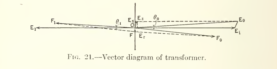
Theory and Calculation of Alternating Current Phenomena, Chapter V, printed page 30, PDF page 58; Fig. 21

Open crop - verification queue

acp-fig-22-rectangular-components

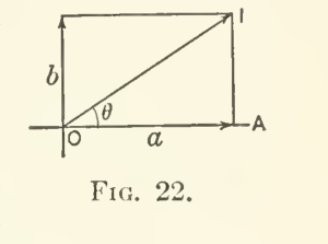
Theory and Calculation of Alternating Current Phenomena, Chapter V, printed page 31, PDF page 59; Fig. 22

Open crop - verification queue

acp-fig-23-resultant-components

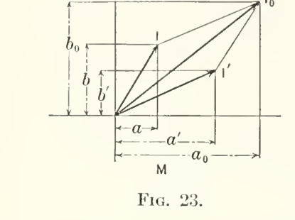
Theory and Calculation of Alternating Current Phenomena, Chapter V, printed page 32, PDF page 60; Fig. 23

Open crop - verification queue

acp-fig-24-quarter-period-rotation

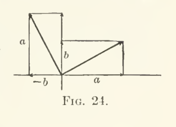
Theory and Calculation of Alternating Current Phenomena, Chapter V, printed page 33, PDF page 61; Fig. 24

Open crop - verification queue

Modern Guide Diagrams Keyed To This Source

Rotating Magnetic Field From Quadrature Fluxes

Modern reading aid for induction-machine field language in AC and Theoretical Elements sources.

symbolic-method, magnetism, phase, induction-motor

Open SVG - recreated visual index

Admittance Plane

Modern reading aid for conductance, susceptance, and reciprocal impedance.

admittance, conductance, susceptance, symbolic-method

Open SVG - recreated visual index

Hysteresis Loss Law

Modern reading aid for the Steinmetz law and magnetic energy loss per cycle.

hysteresis, magnetic-loss, effective-resistance

Open SVG - recreated visual index

Engineering Number Plane

Modern reading aid for number, direction, and symbolic calculation in Engineering Mathematics.

complex-quantities, number, symbolic-method

Open SVG - recreated visual index

AC Symbolic Method Redraw Sheet

Modern redraw sheet for rectangular components, resultant addition, and quarter-period j rotation.

symbolic-method, complex-quantities, phasor, operator-j

Open SVG - recreated visual index

Phasor And Symbolic Method

Modern reading aid for vector and complex-number representation of alternating quantities.

symbolic-method, complex-quantities, phase, phasor

Open SVG - recreated visual index

Hysteresis Loop

Modern guide for magnetic lag, loop area, and energy loss per cycle.

hysteresis, magnetism, magnetic-loss, effective-resistance

Open SVG - recreated visual index

Impedance And Reactance Triangle

Modern guide for resistance, reactance, impedance, phase angle, and symbolic quantities.

impedance, reactance, power-factor, symbolic-method

Open SVG - recreated visual index

Candidate Figure References

Candidate	Caption lead	Section	Routes
theory-calculation-alternating-current-phenomena-fig-006 Fig. 6	maximum variation of the sine is equal to the variation of the Fig. 6. Fig. 7.	Chapter 2: Instantaneous Values And Integral Values	source workbench
theory-calculation-alternating-current-phenomena-fig-007 Fig. 7	Fig. 6. Fig. 7. corresponding arc, and consequently the maximum variation of	Chapter 2: Instantaneous Values And Integral Values	source workbench
theory-calculation-alternating-current-phenomena-fig-010 Fig. 10	21 Fig. 10. phase angle — /3’ = — (a’ — ??]) = 10 A, and the equations of	Chapter 4: Vector Representation	source workbench
theory-calculation-alternating-current-phenomena-fig-016 Fig. 16	^E, Fig. 16. Fig. 17.	Chapter 4: Vector Representation	source workbench
theory-calculation-alternating-current-phenomena-fig-017 Fig. 17	Fig. 16. Fig. 17. the current by the angle, Q. The voltage consumed by the resist-	Chapter 4: Vector Representation	source workbench
theory-calculation-alternating-current-phenomena-fig-019 Fig. 19	Ei-< «; Fig. 19. The primary impressed e.m.f., Ep, must thus consist of the three components OEi, OEr, and OE^, and is, therefore, their	Chapter 4: Vector Representation	source workbench
theory-calculation-alternating-current-phenomena-fig-024 Fig. 24	33 Fig. 24. polar coordinates by a vector of opposite direction, and denoted	Chapter 5: Symbolic Method	source workbench
theory-calculation-alternating-current-phenomena-fig-025 Fig. 25	,,U— — L Fig. 25. Fig. 26.	Chapter 6: Topographic Method	source workbench
theory-calculation-alternating-current-phenomena-fig-026 Fig. 26	Fig. 25. Fig. 26. in the opposite direction, from terminal B to terminal A in op-	Chapter 6: Topographic Method	source workbench
theory-calculation-alternating-current-phenomena-fig-029 Fig. 29	NON-INDUCTIVE LOAD Fig. 29. Fig. 30.	Chapter 6: Topographic Method	source workbench
theory-calculation-alternating-current-phenomena-fig-030 Fig. 30	Fig. 29. Fig. 30. these currents are represented in Fig. 29 by the vectors 01 1 =	Chapter 6: Topographic Method	source workbench
theory-calculation-alternating-current-phenomena-fig-031 Fig. 31	CAPACIir AND RESISTANCE Fig. 31. Fig. 32.	Chapter 6: Topographic Method	source workbench
theory-calculation-alternating-current-phenomena-fig-032 Fig. 32	Fig. 31. Fig. 32. triangle, Ei^E^^Ez^, the voltages at the receiver’s circuit, Ei, E2,	Chapter 6: Topographic Method	source workbench
theory-calculation-alternating-current-phenomena-fig-033 Fig. 33	RESISTANCE AND LEAKAGE Fig. 33. 16 I TRANSMISSION	Chapter 6: Topographic Method	source workbench
theory-calculation-alternating-current-phenomena-fig-034 Fig. 34	90” LAG Fig. 34. and generator currents, /i”, 72°, I^, over the topographical char-	Chapter 6: Topographic Method	source workbench
theory-calculation-alternating-current-phenomena-fig-035 Fig. 35	RESISTANCE AND LEAKAGE Fig. 35. their difference of phase are plotted in Fig. 35 in rectangular	Chapter 6: Topographic Method	source workbench
theory-calculation-alternating-current-phenomena-fig-037 Fig. 37	represented by an increase of angle B in counter-clockwise rota- FiG. 37 tion. That is, the positive direction, or increase of time, is	Chapter 7: Polar Coordinates And Polar Diagrams	source workbench
theory-calculation-alternating-current-phenomena-fig-041 Fig. 41	^i Fig. 41. Fig. 42.	Chapter 7: Polar Coordinates And Polar Diagrams	source workbench
theory-calculation-alternating-current-phenomena-fig-042 Fig. 42	Fig. 41. Fig. 42. then appear in the vector representation of the time diagram or	Chapter 7: Polar Coordinates And Polar Diagrams	source workbench
theory-calculation-alternating-current-phenomena-fig-043 Fig. 43	E^-^ Fig. 43. Fig. 45.	Chapter 7: Polar Coordinates And Polar Diagrams	source workbench
theory-calculation-alternating-current-phenomena-fig-045 Fig. 45	Fig. 43. Fig. 45. lagging behind the voltage:	Chapter 7: Polar Coordinates And Polar Diagrams	source workbench
theory-calculation-alternating-current-phenomena-fig-046 Fig. 46	then means: Fig. 46. POLAR COORDINATES AND POLAR DIAGRAMS 51	Chapter 7: Polar Coordinates And Polar Diagrams	source workbench
theory-calculation-alternating-current-phenomena-fig-048 Fig. 48	^ Fig. 48. R’	Chapter 7: Polar Coordinates And Polar Diagrams	source workbench
theory-calculation-alternating-current-phenomena-fig-049 Fig. 49	7 1.8 Fig. 49. The sign in the complex expression of admittance is always opposite to that of impedance; this is obvious, since if the cur-	Chapter 8: Admittance, Conductance, Susceptance	source workbench
theory-calculation-alternating-current-phenomena-fig-051 Fig. 51	Eo E Fig. 51. M	Chapter 9: Circuits Containing Resistance, Inductive Reactance, And Condensive Reactance	source workbench
theory-calculation-alternating-current-phenomena-fig-052 Fig. 52	Eo Fig. 52. Fig. 53.	Chapter 9: Circuits Containing Resistance, Inductive Reactance, And Condensive Reactance	source workbench
theory-calculation-alternating-current-phenomena-fig-053 Fig. 53	Fig. 52. Fig. 53. 2. Reactance in Series with a Circuit	Chapter 9: Circuits Containing Resistance, Inductive Reactance, And Condensive Reactance	source workbench
theory-calculation-alternating-current-phenomena-fig-054 Fig. 54	ohms inductance-’— reactance-^condensance Fig. 54. E^, are shown for various conditions of a receiver circuit and	Chapter 9: Circuits Containing Resistance, Inductive Reactance, And Condensive Reactance	source workbench
theory-calculation-alternating-current-phenomena-fig-055 Fig. 55	0 Fig. 55. Fig. 56.	Chapter 9: Circuits Containing Resistance, Inductive Reactance, And Condensive Reactance	source workbench
theory-calculation-alternating-current-phenomena-fig-056 Fig. 56	Fig. 55. Fig. 56. Fig. 57.	Chapter 9: Circuits Containing Resistance, Inductive Reactance, And Condensive Reactance	source workbench
theory-calculation-alternating-current-phenomena-fig-057 Fig. 57	Fig. 56. Fig. 57. is, the current and e.m.f. in the supply circuit are in phase with	Chapter 9: Circuits Containing Resistance, Inductive Reactance, And Condensive Reactance	source workbench
theory-calculation-alternating-current-phenomena-fig-058 Fig. 58	^w=+90 80 70 60 50 40 30 20 10 0 10 20 30 40 50 60 70 80 90 degrees lag-«- phase difference in consumer circuit-*- lead Fig. 58. In Figs. 59 and 60, the same curves are plotted as in Fig. 58, but in Fig. 59 with the r…	Chapter 9: Circuits Containing Resistance, Inductive Reactance, And Condensive Reactance	source workbench
theory-calculation-alternating-current-phenomena-fig-059 Fig. 59	+1 +.9 +.8 +.7 +.6 +.5 +.4 +.3 +.2 +.1 0 -.1 -.2 -.3 -.4 -.5 -.6 reactance of consumer circuit Fig. 59. -.7 -.8 -.9-10	Chapter 9: Circuits Containing Resistance, Inductive Reactance, And Condensive Reactance	source workbench
theory-calculation-alternating-current-phenomena-fig-060 Fig. 60	_ resistance of . consumer circuit Fig. 60. ,7 .6 .5 .4 .3 .2 .1 .0	Chapter 9: Circuits Containing Resistance, Inductive Reactance, And Condensive Reactance	source workbench
theory-calculation-alternating-current-phenomena-fig-061 Fig. 61	1. .9 .8 .7 .6 .5 ,4 .3 .2 .1 0 -.1 -.2 -.3 -.1 -.5 -.6 -.7 -.8 -.9-L X — ^ Fig. 61. E	Chapter 9: Circuits Containing Resistance, Inductive Reactance, And Condensive Reactance	source workbench
theory-calculation-alternating-current-phenomena-fig-062 Fig. 62	tro Fig. 62. Fig. 63.	Chapter 9: Circuits Containing Resistance, Inductive Reactance, And Condensive Reactance	source workbench
theory-calculation-alternating-current-phenomena-fig-063 Fig. 63	Fig. 62. Fig. 63. 72	Chapter 9: Circuits Containing Resistance, Inductive Reactance, And Condensive Reactance	source workbench
theory-calculation-alternating-current-phenomena-fig-065 Fig. 65	loss of power. Fig. 65. Then, if Eo = impressed e.m.f., the current in receiver circuit is	Chapter 9: Circuits Containing Resistance, Inductive Reactance, And Condensive Reactance	source workbench
theory-calculation-alternating-current-phenomena-fig-067 Fig. 67	1 Fig. 67. 5. Constant Potential — Constant-current Transformation	Chapter 9: Circuits Containing Resistance, Inductive Reactance, And Condensive Reactance	source workbench
theory-calculation-alternating-current-phenomena-fig-068 Fig. 68	supply, and inversely. Fig. 68 The generation of alternating-current electric power almost always takes place at constant potential. For some purposes,	Chapter 9: Circuits Containing Resistance, Inductive Reactance, And Condensive Reactance	source workbench
theory-calculation-alternating-current-phenomena-fig-072 Fig. 72	0 Fig. 72. .03 ,03 M. .05 .00 .07 .OS	Chapter 10: Resistance And Reactance Of Transmission	source workbench
theory-calculation-alternating-current-phenomena-fig-076 Fig. 76	» Fig. 76. 10 20 30 10 50 60 7.0 .80 90 100	Chapter 10: Resistance And Reactance Of Transmission	source workbench
theory-calculation-alternating-current-phenomena-fig-077 Fig. 77	AMPERES LOAD « l Fig. 77. and the leading quadrature component of current required to compensate for the line reactance x at maximum current, im, is	Chapter 11: Phase Control	source workbench
theory-calculation-alternating-current-phenomena-fig-078 Fig. 78	::} Fig. 78. 87. Equation (28) shows that there are two values of x: Xi and X2; and corresponding thereto two values of 60:^01 and 602,	Chapter 11: Phase Control	source workbench
theory-calculation-alternating-current-phenomena-fig-081 Fig. 81	^ Fig. 81. The general character of these current waves is, that the maxi-	Chapter 12: Effective Resistance And Reactance	source workbench
theory-calculation-alternating-current-phenomena-fig-082 Fig. 82	then Fig. 82. — X^	Chapter 12: Effective Resistance And Reactance	source workbench
theory-calculation-alternating-current-phenomena-fig-086 Fig. 86	n = NUMBER OF TURNS Fig. 86. 350	Chapter 12: Effective Resistance And Reactance	source workbench
theory-calculation-alternating-current-phenomena-fig-087 Fig. 87	/ = FREQUENCY Fig. 87. 400	Chapter 12: Effective Resistance And Reactance	source workbench
theory-calculation-alternating-current-phenomena-fig-088 Fig. 88	200 250 Fig. 88. 300	Chapter 12: Effective Resistance And Reactance	source workbench
theory-calculation-alternating-current-phenomena-fig-089 Fig. 89	/=CYCLES Fig. 89. 300	Chapter 12: Effective Resistance And Reactance	source workbench
theory-calculation-alternating-current-phenomena-fig-090 Fig. 90	n=NUMBER OF TURNS Fig. 90. 350	Chapter 12: Effective Resistance And Reactance	source workbench
theory-calculation-alternating-current-phenomena-fig-092 Fig. 92	magnetic flux inclosed by the zone is SuV. Fig. 92. Hence, the e.m.f. generated in this zone is	Chapter 13: Foucault Or Eddy Currents	source workbench
theory-calculation-alternating-current-phenomena-fig-093 Fig. 93	93. Fig. 93. 110. Demagnetizing, or screening effect of eddy currents.	Chapter 13: Foucault Or Eddy Currents	source workbench
theory-calculation-alternating-current-phenomena-fig-094 Fig. 94	du Fig. 94. The current inclosed by this zone is /„	Chapter 13: Foucault Or Eddy Currents	source workbench
theory-calculation-alternating-current-phenomena-fig-096 Fig. 96	^ m Fig. 96. )J	Chapter 14: Dielectric Losses	source workbench
theory-calculation-alternating-current-phenomena-fig-097 Fig. 97	’ m Fig. 97. throughout the field section, but the voltage gradient in the	Chapter 14: Dielectric Losses	source workbench
theory-calculation-alternating-current-phenomena-fig-098 Fig. 98	do so. Fig. 98. Fig. 99.	Chapter 14: Dielectric Losses	source workbench
theory-calculation-alternating-current-phenomena-fig-099 Fig. 99	Fig. 98. Fig. 99. h’5	Chapter 14: Dielectric Losses	source workbench
theory-calculation-alternating-current-phenomena-fig-100 Fig. 100	JTTTTTTTTTTTTTTTTTTTTTTT- Fig. 100. In this case the intensity as well as phase of the current, and consequently of the counter e.m.f. of inductive reactance and	Chapter 15: Distributed Capacity, Inductance, Resistance, And Leakage	source workbench
theory-calculation-alternating-current-phenomena-fig-101 Fig. 101	iEo Fig. 101. Denoting in Fig. 101.	Chapter 15: Distributed Capacity, Inductance, Resistance, And Leakage	source workbench